MSnbase: centroiding of profile-mode MS data

Abstract

This vignette describes the use of the MSnbase package for centroiding of profile-mode mass spectrometry data.

Introduction

Mass spectrometry measures data in so called profile mode, were the signal corresponding to a specific ion is distributed around the ion’s actual m/z value (Smith et al. 2014). The accuracy of that signal depends on the resolution and settings of the instrument. Profile mode data can be processed into centroid data by retaining only a single, representative value, typically the local maximum of the distribution of data points. This centroiding substantially reduces the amount of data without much loss of information. Certain algorithms, such as the centWave method in the xcms package for chromatographic peak detection in LC-MS experiments or proteomics search engines that match MS2 spectra to peptides, require the data to be in centroid mode. In this vignette, we will focus on metabolomics data.

Many manufacturers apply centroiding of the profile data, either directly during the acquisition or immediately thereafter so that the user immediately receives processed data. Alternatively, third party software, such as msconvert from the proteowizard suite (Chambers et al. 2012) allow to apply various data centroiding algorithms, including vendor methods. In some cases however, the software provided by some vendors generate centroided data of poor quality. MSnbase also provides some functionality to perform centroiding of profile MS data. These processed data can then be further quantified or analysed within R or serialised to mzML files, and used as input for other software.

Centroiding of profile-mode MS data

In this vignette we use a subset of a metabolomics profile-mode LC-MS data of pooled human serum samples measured on a AB Sciex TripleTOF 5600+ mass spectrometer (the employed chromatography was a hydrophilic interaction high-performance liquid chromatography (HILIC HPLC)). The mzML file contains profile mode data for an m/z range from 105 to 130 and a retention time from 0 to 240 seconds. For more details on the sample see ?msdata::sciexdata. Below we load the required packages and read the MS data.

library("MSnbase")
library("msdata")
library("magrittr")

fl <- dir(system.file("sciex", package = "msdata"), full.names = TRUE)[2]
basename(fl)

## [1] "20171016_POOL_POS_3_105-134.mzML"

data_prof <- readMSData(fl, mode = "onDisk", centroided = FALSE)

We next extract the profile MS data for the [M+H]+ adduct of serine with the expected m/z of 106.049871. We thus filter the data_prof object using an m/z range containing the signal for the metabolite and a retention time window from 175 to 187 seconds corresponding to the time when the analyte elutes from the LC.

## Define the mz and retention time ranges
serine_mz <- 106.049871
mzr <- c(serine_mz - 0.01, serine_mz + 0.01)
rtr <- c(175, 187)

## Filtering the object
serine <- data_prof %>%
    filterRt(rtr) %>%
    filterMz(mzr)

We can now plot the profile MS data for serine.

plot(serine, type = "XIC")
abline(h = serine_mz, col = "red", lty = 2)

MS profile data for serine. Upper panel shows the base peak chromatogram (BPC), lower panel the individual signals in the retention time - m/z space. The horizontal dashed red line indicates the theoretical m/z of the [M+H]+ adduct of serine.

The lower panel in the plot above shows all the individual signal intensities measured by the mass spectrometer over the retention time and the m/z ranges of interest. The upper panel displays the base peak chromatogram (BPC), which represents the maximum signal (across the range of m/z values) for each discrete retention time. The rows of points in this lower panel indicate the resolution of the mass spectrometer while the columns of data points (i.e. the data collected for a discrete retention time point) represents the signal for the ion in one spectrum.

Below we plot the signal for one of of the 43 spectra containing signal for serine, the one at retention time 181.07

plot(serine[[22]])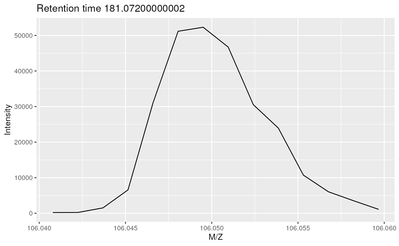

On of the spectra for serine in profile mode.

The MS instrument recorded a signal along the m/z range in discrete intervals (which depend on the resolution of the instrument). The profile-mode signal of the serine ion at the respective retention time (the mass peak) consists therefore of multiple intensities that follow approximately a gaussian distribution.

As described in the introduction, centroiding aims to reduce this signal distribution to a single representative intensity, a single data point, for the ion in a spectrum. The simplest approach selects the largest intensity for each mass peak and report its intensity and m/z value. This can be done using the pickPeaks method with default parameters as shown below.

data_cent <- data_prof %>%
    pickPeaks()

serine_cent <- data_cent %>%
    filterRt(rtr) %>%
    filterMz(mzr)

## Plot the centroided data for serine
plot(serine_cent, type = "XIC")
abline(h = serine_mz, col = "red", lty = 2)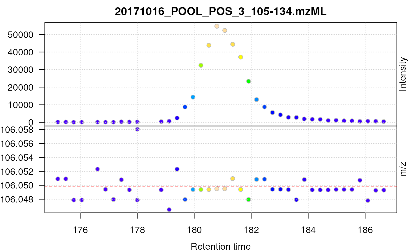

Centroided data for serine.

After centroiding the data consists of a single intensity for each mass peak. In the example above the centroids from consecutive scans do however not have the same m/z value, but they fluctuate between the discrete m/z values defined by the instruments’s resolution. For lower intensity signals this variation can be substantial.

To further illustrate this, we plot below the centroided signal for the [M+H]+ ion of proline.

prol_mz <- 116.070608
prol_mzr <- c(prol_mz - 0.01, prol_mz + 0.01)
prol_rtr <- c(165, 175)

proline <- data_prof %>%
    pickPeaks() %>%
    filterRt(prol_rtr) %>%
    filterMz(prol_mzr)

plot(proline, type = "XIC")
abline(h = prol_mz, col = "red", lty = 2)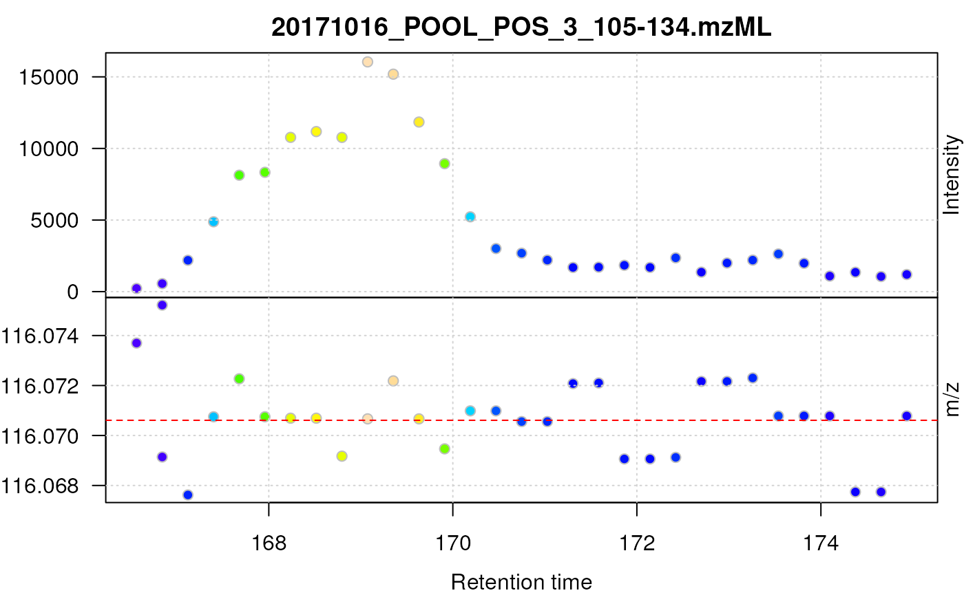

Centroided data for proline.

For proline, the centroids jump between 3 bins of m/z values in consecutive scans and the chromatographic data does not show a nice, regular peak shape. Additional data processing, such as data smoothing prior to centroiding and/or refining the centroid’s m/z can reduce these effects and improve overall data quality as we will see in the next section.

Improving the signal quality

While the simple centroiding using pickPeaks as described in the previous section might be sufficient for many experiments and setups, MS data smoothing and refinement of the identified centroids’ m/z values can improve data quality.

Data smoothing

Raw mass spectrometry data is usually smoothed in m/z dimension by applying e.g. a Savitzky-Golay filter (Savitzky and Golay 1964) which reduces the noise and hence improves data quality. Below we use the smooth method to apply a Savitzky-Golay filter with a half-window size of 4 to the data within each spectrum (see ?smooth for more details on the parameters).

data_sg <- data_prof %>%
    smooth(method = "SavitzkyGolay", halfWindowSize = 4L)

We next apply the simple peak picking on the smoothed data, filter the desired retention time and m/z ranges, and subsequently plot the such centroided data for serine.

data_sg_cent <- data_sg %>%
    pickPeaks %>%
    filterRt(rtr) %>%
    filterMz(mzr)

## Plot the centroided data for serine
plot(data_sg_cent, type = "XIC")
abline(h = serine_mz, col = "red", lty = 2)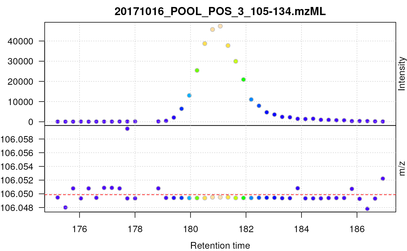

Centroided data for serine after smoothing with a Savitzky-Golay filter.

Smoothing the raw data prior to peak picking improved the quality of the centroided data of serine as well as proline as can be seen below.

prol_sg_cent <- data_sg %>%
    pickPeaks %>%
    filterRt(prol_rtr) %>%
    filterMz(prol_mzr)

plot(prol_sg_cent, type = "XIC")
abline(h = prol_mz, col = "red", lty = 2)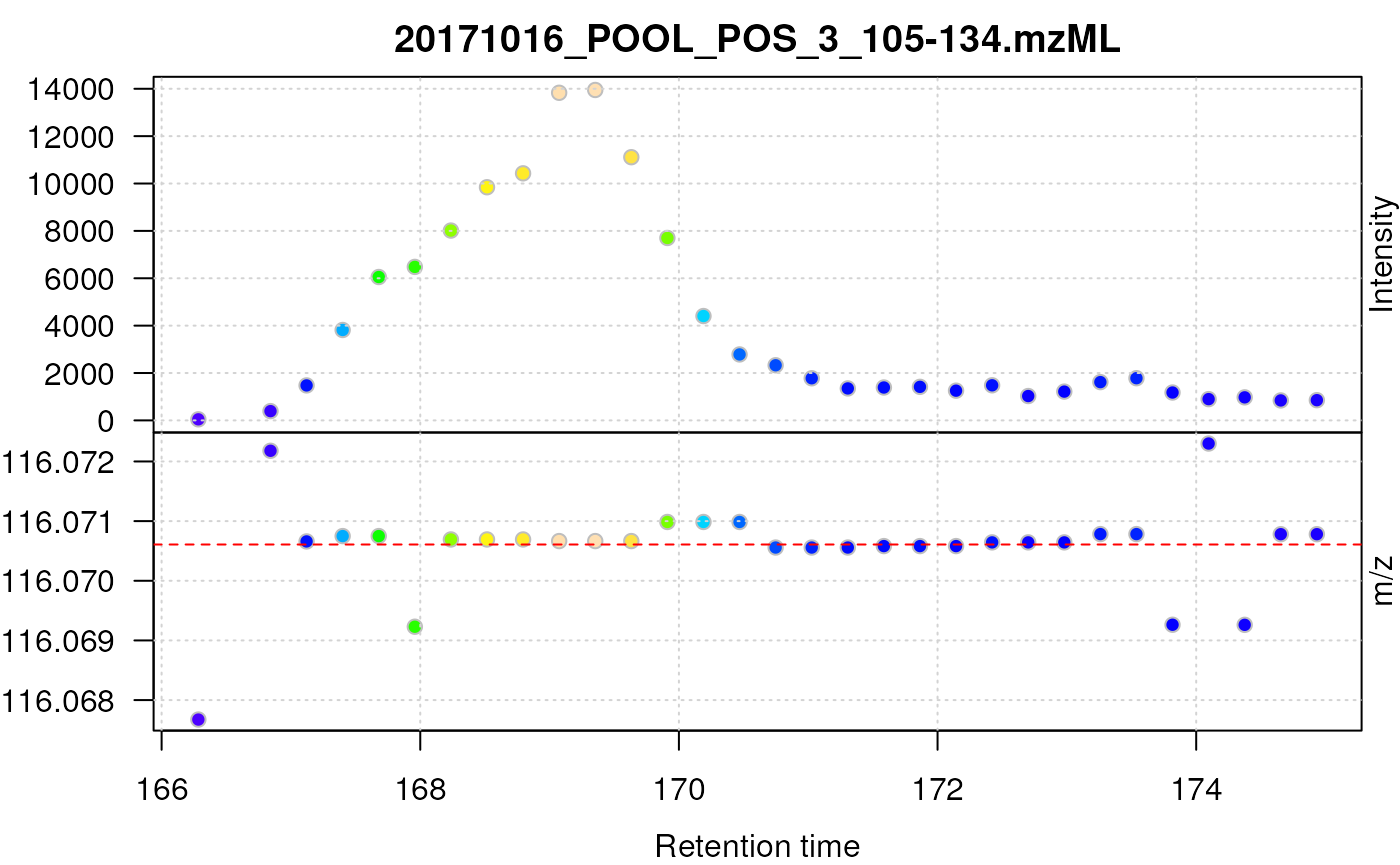

Centroided data for proline after smoothing with a Savitzky-Golay filter.

The smoothed centroided data for proline still show a systematic deviation of m/z values as well as poor chromatographic data.

In addition to smoothing the signal in m/z dimension, we can also smooth the signal along the retention time dimension using the combineSpectraMovingWindow function. This function aggregates signal for the same m/z value from neighbouring spectra in a moving window approach, thus smoothing the chromatographic data (by replacing the intensity in the middle spectrum by the average signal of all intensities for the m/z in the spectra within the defined window). To reduce the run-time of the example we apply the smoothing only to the profile-mode data for a retention time window containing proline (in a real data analysis this should be performed on the full data).

## Subset to the data for proline, smooth it in rt dimension and
## perform the centroiding
proline_c_cent <- data_prof %>%
    filterRt(prol_rtr) %>%
    combineSpectraMovingWindow() %>%
    pickPeaks() %>%
    filterMz(prol_mzr)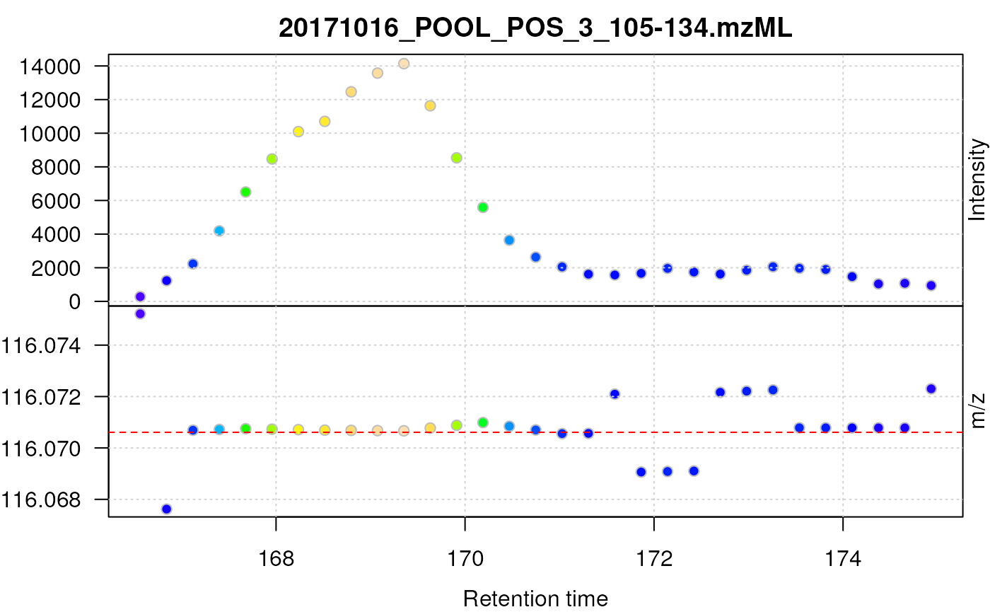

plot(proline_c_cent, type = "XIC")
abline(h = prol_mz, col = "red", lty = 2)

Centroided data for proline after smoothing in retention time dimension.

As can be seen above, smoothing in retention time dimension improves the chromatographic peak shape of proline.

Note however that, to combine data from multiple spectra, the combineSpectraMovingWindow function has to first load the full data into memory (i.e. it converts the OnDiskMSnExp object into a MSnExp object) and that it returns also a MSnExp object. In a real use case it is thus advisable to apply combineSpectraMovingWindow separately on each file of an experiment and to export the results as an mzML file using the writeMSData method.

Refinement of the centroid’s m/z values

Thus far we applied only a simple peak picking strategy, but the pickPeaks method allows also to refine the identified centroid’s m/z value by considering also the signal from the full, or parts of the, mass peak. Currently two methods are implemented, descendPeak and kNeighbors that can be selected by passing either refineMz = "descendPeak" or refineMz = "kNeighbors" to the pickPeaks method. The m/z value of the reported centroid is calculated using an intensity-weighted mean of m/z-intensity values from the mass peak. This can improve the accuracy of the reported m/z values. The two methods differ only in the way in which the peak area for the final calculation is defined: kNeighbors takes the k m/z-intensity pairs (default k = 2) left and right of the centroid and descendPeak walks, on both sides from the centroid, down until the signal is below signalPercentage% of the centroid’s intensity (by default 33%), or until the signal increases again. All m/z intensity pairs within this range are used for the weighted average calculation of the centroid’s m/z value.

## Use pickPeaks with descendPeak m/z refinement
data_sg_cent_mz <- data_sg %>%
    pickPeaks(refineMz = "descendPeak")

Below we first extract the data for serine and then plot the smoothed and centroided data without and with m/z refinement.

## Extract the data for serine
serine_sg_cent <- data_sg_cent %>%
    filterRt(rtr) %>%
    filterMz(mzr)

serine_sg_cent_mz <- data_sg_cent_mz %>%
    filterRt(rtr) %>%
    filterMz(mzr)

## Plot the data
layout(matrix(1:4, ncol = 2))
## No m/z refinement
plot(serine_sg_cent, type = "XIC", layout = NULL)
abline(h = serine_mz, col = "red", lty = 2)
abline(v = rtime(serine_sg_cent)[22], col = "red", lty = 3)
## With m/z refinement
plot(serine_sg_cent_mz, type = "XIC", layout = NULL)
abline(h = serine_mz, col = "red", lty = 2)
abline(v = rtime(serine_sg_cent_mz)[22], col = "red", lty = 3)

Smoothed and centroided data for serine without (left) and with m/z refinement (right). The horizontal red dashed line indicates the theoretical m/z for the [M+H]+ ion and the vertical red dotted line the position of the largest signal for serine.

As shown above (right), the accuracy of the centroided data with m/z refinement was improved, where the difference between the largest signal centroids’ m/z value and the theoretical m/z value for the [M+H]+ ion of serine is reduced.

For the simple peak picking on raw data the difference is:

## only centroided
mz(filterMz(filterRt(data_cent, rtr), mzr))[[22]] - serine_mz

## [1] -0.0003682412

Smoothing already improves the accuracy:

## smoothed and centroided
mz(serine_sg_cent)[[22]] - serine_mz

## [1] -0.0003682412

And refining the m/z value during the centroiding can improve accuracy even more:

## smoothed and centroided with m/z refinement
mz(serine_sg_cent_mz)[[22]] - serine_mz

## [1] -0.0001703475

Similarly, the m/z refinement also improved the accuracy for proline.

proline_sg_cent <- data_prof %>%
    smooth(method = "SavitzkyGolay", halfWindowSize = 4L) %>%
    pickPeaks() %>%
    filterRt(prol_rtr) %>%
    filterMz(prol_mzr)

proline_sg_cent_mz <- data_prof %>%
    smooth(method = "SavitzkyGolay", halfWindowSize = 4L) %>%
    pickPeaks(refineMz = "descendPeak") %>%
    filterRt(prol_rtr) %>%
    filterMz(prol_mzr)

layout(matrix(1:4, ncol = 2))
plot(proline_sg_cent, type = "XIC", layout = NULL)
abline(h = prol_mz, col = "red", lty = 2)
abline(v = rtime(proline_sg_cent_mz)[16], col = "red", lty = 3)

plot(proline_sg_cent_mz, type = "XIC", layout = NULL)
abline(h = prol_mz, col = "red", lty = 2)
abline(v = rtime(proline_sg_cent_mz)[16], col = "red", lty = 3)

Smoothed and centroided data for proline without (left) and with m/z refinement (right). The horizontal red dashed line indicates the theoretical m/z for the [M+H]+ ion and the vertical red dotted line the position of the maximum signal.

The difference between the m/z of the centroid with the largest signal and the theoretical m/z for the [M+H]+ ion of proline is shown below.

## only centroiding
mz(filterMz(filterRt(data_cent, prol_rtr), prol_mzr))[[16]] - prol_mz

## [1] 0.001577028

## smoothed and centroided
mz(proline_sg_cent)[[16]] - prol_mz

## [1] 5.75261e-05

## smoothed and centroided with m/z refinement
mz(proline_sg_cent_mz)[[16]] - prol_mz

## [1] -3.241556e-05

Summarizing, smoothing raw profile MS data, e.g. by applying a Savitzky-Golay filter, improves quality considerably. Additional smoothing in retention time dimension can be advantageous too, specifically for the chromatographic peak shape. Accuracy can be further improved for smoothed profile MS data by refining the m/z value of the identified centroids.

References

Chambers, M C, B Maclean, R Burke, D Amodei, D L Ruderman, S Neumann, L Gatto, et al. 2012. “A Cross-Platform Toolkit for Mass Spectrometry and Proteomics.” Nat Biotechnol 30 (10): 918–20. https://doi.org/10.1038/nbt.2377.

Savitzky, Abraham, and M J E Golay. 1964. “Smoothing and Differentiation of Data by Simplified Least Squares Procedures.” Analytical Chemistry 36 (8): 1627–39.