Generate an average MSnSet

Given a list of MSnSet instances, typically representing replicated experiments, the function returns an average MSnSet.

averageMSnSet(x, avg = function(x) mean(x, na.rm = TRUE), disp = npcv)

Arguments

x

A list of valid MSnSet instances to be averaged.

avg

The averaging function. Default is the mean after removing missing values, as computed by function(x) mean(x, na.rm = TRUE).

disp

The disperion function. Default is an non-parametric coefficient of variation that replaces the standard deviation by the median absolute deviation as computed by mad(x)/abs(mean(x)). See npcv for details. Note that the mad of a single value is 0 (as opposed to NA for the standard deviation, see example below).

Value

A new average MSnSet.

Details

This function is aimed at facilitating the visualisation of replicated experiments and should not be used as a replacement for a statistical analysis.

The samples of the instances to be averaged must be identical but can be in a different order (they will be reordered by default). The features names of the result will correspond to the union of the feature names of the input MSnSet instances. Each average value will be computed by the avg function and the dispersion of the replicated measurements will be estimated by the disp function. These dispersions will be stored as a data.frame in the feature metadata that can be accessed with fData(.)$disp. Similarly, the number of missing values that were present when average (and dispersion) were computed are available in fData(.)$disp.

Currently, the feature metadata of the returned object corresponds the the feature metadata of the first object in the list (augmented with the missing value and dispersion values); the metadata of the features that were missing in this first input are missing (i.e. populated with NAs). This may change in the future.

See also

compfnames to compare MSnSet feature names.

Author

Laurent Gatto

Examples

library("pRolocdata")
## 3 replicates from Tan et al. 2009
data(tan2009r1)
data(tan2009r2)
data(tan2009r3)
x <- MSnSetList(list(tan2009r1, tan2009r2, tan2009r3))
avg <- averageMSnSet(x)
dim(avg)
#> [1] 1311    4
head(exprs(avg))
#>             X114      X115      X116      X117
#> P20353 0.3605000 0.3035000 0.2095000 0.1265000
#> P53501 0.4299090 0.1779700 0.2068280 0.1852625
#> Q7KU78 0.1704443 0.1234443 0.1772223 0.5290000
#> P04412 0.2567500 0.2210000 0.3015000 0.2205000
#> Q7KJ73 0.2160000 0.1830000 0.3420000 0.2590000
#> Q7JZN0 0.0965000 0.2509443 0.4771667 0.1750557
head(fData(avg)$nNA)
#>        X114 X115 X116 X117
#> P20353    1    1    1    1
#> P53501    1    1    1    1
#> Q7KU78    0    0    0    0
#> P04412    1    1    1    1
#> Q7KJ73    2    2    2    2
#> Q7JZN0    0    0    0    0
head(fData(avg)$disp)
#>               X114      X115        X116       X117
#> P20353 0.076083495 0.1099127 0.109691169 0.14650198
#> P53501 0.034172542 0.2640556 0.005139653 0.17104568
#> Q7KU78 0.023198743 0.4483795 0.027883087 0.04764499
#> P04412 0.053414021 0.2146751 0.090972139 0.27903810
#> Q7KJ73 0.000000000 0.0000000 0.000000000 0.00000000
#> Q7JZN0 0.007681865 0.1959534 0.097873350 0.06210542
## using the standard deviation as measure of dispersion
avg2 <-averageMSnSet(x, disp = sd)
head(fData(avg2)$disp)
#>              X114       X115       X116       X117
#> P20353         NA         NA         NA         NA
#> P53501         NA         NA         NA         NA
#> Q7KU78 0.03158988 0.04750696 0.01033500 0.04667976
#> P04412         NA         NA         NA         NA
#> Q7KJ73         NA         NA         NA         NA
#> Q7JZN0 0.02121910 0.04160155 0.08447534 0.04988318
## keep only complete observations, i.e proteins 
## that had 0 missing values for all samples
sel <- apply(fData(avg)$nNA, 1 , function(x) all(x == 0))
avg <- avg[sel, ]
disp <- rowMax(fData(avg)$disp)
library("pRoloc")
#> Loading required package: MLInterfaces
#> Loading required package: annotate
#> Loading required package: AnnotationDbi
#> Loading required package: XML
#> 
#> Attaching package: ‘annotate’
#> The following object is masked from ‘package:mzR’:
#> 
#>     nChrom
#> Loading required package: cluster
#> Loading required package: BiocParallel
#> 
#> This is pRoloc version 1.43.2 
#>   Visit https://lgatto.github.io/pRoloc/ to get started.
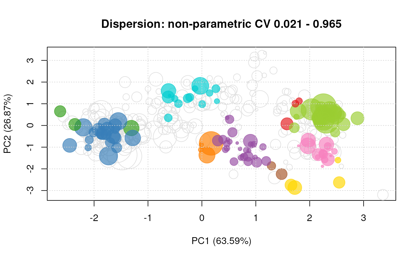
setStockcol(paste0(getStockcol(), "AA"))
plot2D(avg, cex = 7.7 * disp)
title(main = paste("Dispersion: non-parametric CV",
                   paste(round(range(disp), 3), collapse = " - ")))