Plotting a 'Spectrum' vs another 'Spectrum' object.

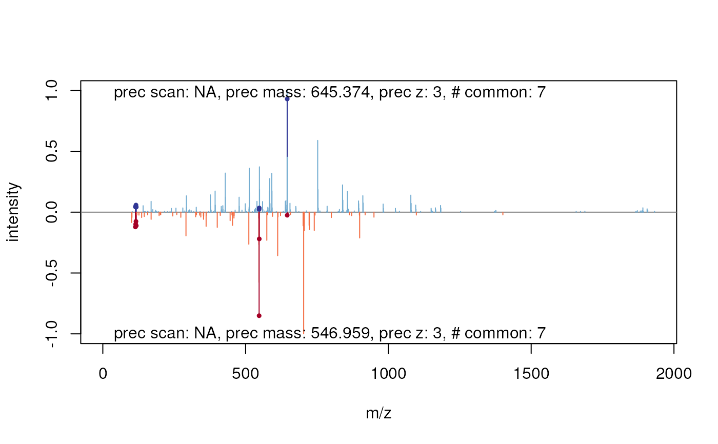
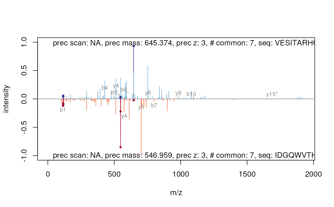
These method plot mass spectra MZ values against the intensities as line plots. The first spectrum is plotted in the upper panel and the other in upside down in the lower panel. Common peaks are drawn in a slightly darker colour. If a peptide sequence is provided it automatically calculates and labels the fragments.

Arguments

x

Object of class "Spectrum" .

y

Object of class "Spectrum" .

...

Further arguments passed to internal functions.

Methods

signature(x = "Spectrum", y = "Spectrum", ...)

Plots two spectra against each other. Common peaks are drawn in a slightly darker colour. The ... arguments are passed to the internal functions. Currently tolerance, relative, sequences and most of the plot.default arguments (like xlim, ylim, main, xlab, ylab, ...) are supported. You could change the tolerance (default 25e-6) and decide whether this tolerance should be applied relative (default relative = TRUE) or absolute (relative = FALSE) to find and colour common peaks. Use a character vector of length 2 to provide sequences which would be used to calculate and draw the corresponding fragments. If sequences are given the type argument (default: type=c("b", "y") specify the fragment types which should calculated. Also it is possible to allow some modifications. Therefore you have to apply a named character vector for modifications where the name corresponds to the one-letter-code of the modified amino acid (default: Carbamidomethyl modifications=c(C=57.02146)). Additional you can specifiy the type of neutralLoss (default: PSMatch::defaultNeutralLoss()). See calculateFragments for details.

There are a lot of graphical arguments available to control the representation of the peaks and fragments. Use peaks.pch to set the character on top of the peaks (default: peaks.pch=19). In a similar way you can set the line width peaks.lwd=1 and the magnification peaks.cex=0.5 of the peaks. The size of the fragment/legend labels could be set using fragments.cex=0.75 or legend.cex respectively. See par for details about graphical parameters in general.

Author

Sebastian Gibb <mail@sebastiangibb.de>

See also

More spectrum plotting available in plot.Spectrum.

More details about fragment calculation: calculateFragments.

Examples

## find path to a mzXML file
file <- dir(system.file(package = "MSnbase", dir = "extdata"),
            full.name = TRUE, pattern = "mzXML$")

## create basic MSnExp
msexp <- readMSData(file, centroided.=FALSE)

## centroid them
msexp <- pickPeaks(msexp)

## plot the first against the second spectrum
plot(msexp[[1]], msexp[[2]])


## add sequence information
plot(msexp[[1]], msexp[[2]], sequences=c("VESITARHGEVLQLRPK",
                                         "IDGQWVTHQWLKK"))



itraqdata2 <- pickPeaks(itraqdata)
(k <- which(fData(itraqdata2)[, "PeptideSequence"] == "TAGIQIVADDLTVTNPK"))
#> [1] 41 42
mzk <- precursorMz(itraqdata2)[k]
zk <- precursorCharge(itraqdata2)[k]
mzk * zk
#>      X46      X47 
#> 2046.175 2045.169 
plot(itraqdata2[[k[1]]], itraqdata2[[k[2]]])