A Grammar of Data Manipulation for Omics Experiments
Laurent Gatto
Source:vignettes/tidies.Rmd
tidies.RmdIntroduction
The tidies package (from to contraction of tidy eSet) implements tidy principles as defined in the tidyverse packages to omics-type data based on the eSet class, with (currently at least for now), an emphasis on quantitative proteomics data.
High throughput data and the eSet class
The motivation to store omics data in dedicated containers is to coordinate the high throughput data (e.g., gene or protein expression), the sample annotation (phenotype data) and the feature annotation (feature data).
A typical omics data structure, as defined by the eSet class, is represented below. It’s main features are
An assay data slot containing the quantitative omics data (expression data), stored as a
matrixand accessible withexprs. Features defined along the rows and samples along the columns.A sample metadata slot containing sample co-variates, stored as an annotated
data.frameand accessible withpData. This data frame is stored with rows representing samples and sample covariate along the columns, and its rows match the expression data columns exactly.A feature metadata slot containing feature co-variates, stored as an annotated
data.frameand accessible withfData. This dataframe’s rows match the expression data rows exactly.
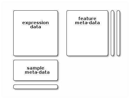
A typical omics data object
The coordinated nature of the high throughput data guarantees that the dimensions of the different slots will always match (i.e the columns in the expression data and then rows in the sample metadata, as well as the rows in the expression data and feature metadata) during data manipulation. The metadata slots can grow additional co-variates (columns) without affecting the other structures.
To illustrate such an omics data container, we’ll make use of the msnset object that comes with the MSnbase package, which contains data for 55 features and 4 samples.
library("MSnbase")
data(msnset)

## Some test sample groups
msnset$group <- c("A", "A", "B", "B")
dim(msnset)
## [1] 55 4The expression data:
head(exprs(msnset))
##     iTRAQ4.114 iTRAQ4.115 iTRAQ4.116 iTRAQ4.117
## X1   1347.6158  2247.3097  3927.6931  7661.1463
## X10   739.9861   799.3501   712.5983   940.6793
## X11 27638.3582 33394.0252 32104.2879 26628.7278
## X12 31892.8928 33634.6980 37674.7272 37227.7119
## X13 26143.7542 29677.4781 29089.0593 27902.5608
## X14  6448.0829  6234.1957  6902.8903  6437.2303
The sample metadata:
pData(msnset)
##               mz reporters group
## iTRAQ4.114 114.1    iTRAQ4     A
## iTRAQ4.115 115.1    iTRAQ4     A
## iTRAQ4.116 116.1    iTRAQ4     B
## iTRAQ4.117 117.1    iTRAQ4     B
The feature metadata:
fData(msnset)[1:10, 1:5]
##     spectrum ProteinAccession                       ProteinDescription
## X1         1              BSA                     bovine serum albumin
## X10       10          ECA1422 glucose-1-phosphate cytidylyltransferase
## X11       11          ECA4030         50S ribosomal subunit protein L4
## X12       12          ECA3882                   chaperone protein DnaK
## X13       13          ECA1364      succinyl-CoA synthetase alpha chain
## X14       14          ECA0871              NADP-dependent malic enzyme
## X15       15          ECA4512                  ATP synthase beta chain
## X16       16          ECA4513                 ATP synthase gamma chain
## X17       17          ECA3969  fumarate reductase flavoprotein subunit
## X18       18          ECA3082            malate:quinone oxidoreductase
##       PeptideSequence file
## X1             NYQEAK    1
## X10   VTLVDTGEHSMTGGR    1
## X11             SPIWR    1
## X12          TAIDDALK    1
## X13            SILINK    1
## X14      DFEVVNNESDPR    1
## X15 EGNDFYHEMTDSNVIDK    1
## X16        VMLQAYDEGR    1
## X17     ANAVVLATGGAGR    1
## X18         VATPEWQSK    1
## all feature variables fvarLabels(msnset)
##  [1] "spectrum"            "ProteinAccession"    "ProteinDescription"
##  [4] "PeptideSequence"     "file"                "retention.time"
##  [7] "precursor.mz"        "precursor.intensity" "charge"
## [10] "peaks.count"         "tic"                 "ionCount"
## [13] "ms.level"            "acquisition.number"  "collision.energy"
Tidy tools
The tidy data definition and tidy tools manifesto lay out the principles that packages in the tidyverse package. tidies isn’t part of the tidyverse, but aims at applying these same principles. The concepts that are relevant for the application to omics data are
Reuse of existing data structures; in this case
eSetobjects, that constitute our tidy omics data.Compose simple functions with the pipe; here we apply the widely used dplyr functions and magrittr
%>%operator. Each of the adapted tidy function to use and return tidyeSetdata.Keep the ability to use existing Bioconductor functions that operate on the
eSetclass; this assumes that these functions are tidy themselves, i.e. that they return aneSetobject.
The tidies package
The goal of this package is to support the dplyr function such as select, filter, group_by, summarise, … direcly on omics data containers described above. The function act on the respective variable and expression slots and preserve the object’s class.
Another approach is to convert the omics objects to tidy tibbles and work direcly with these. This can easily be done with the Bioconductor biobroom package, that will convert the 55 features by 4 samples into a 220 tibble:
library("biobroom")
## Loading required package: broom## Registered S3 methods overwritten by 'biobroom':
## method from
## glance.list broom
## tidy.list broomtidy(msnset, addPheno = TRUE)
## # A tibble: 220 x 6
##    protein sample        mz reporters group  value
##    <chr>   <chr>      <dbl> <fct>     <chr>  <dbl>
##  1 X1      iTRAQ4.114  114. iTRAQ4    A      1348.
##  2 X10     iTRAQ4.114  114. iTRAQ4    A       740.
##  3 X11     iTRAQ4.114  114. iTRAQ4    A     27638.
##  4 X12     iTRAQ4.114  114. iTRAQ4    A     31893.
##  5 X13     iTRAQ4.114  114. iTRAQ4    A     26144.
##  6 X14     iTRAQ4.114  114. iTRAQ4    A      6448.
##  7 X15     iTRAQ4.114  114. iTRAQ4    A       722.
##  8 X16     iTRAQ4.114  114. iTRAQ4    A     10155.
##  9 X17     iTRAQ4.114  114. iTRAQ4    A      2800.
## 10 X18     iTRAQ4.114  114. iTRAQ4    A      4459.
## # … with 210 more rows
Using biobroom::tidy drops the feature data that, sometimes, is important. It is possible to create dataframe that contains these metadata using the following approach. First, combine the expression data and the feature data into a single wide dataframe using ms2df
x <- MSnbase::ms2df(msnset)
which then can be converted to a long, tidy, form with
fv <- fvarLabels(msnset)
library("tidyr")
##
## Attaching package: 'tidyr'
## The following object is masked from 'package:S4Vectors':
##
## expandx <- tidyr::pivot_longer(x, names_to = "sample", values_to = "exprs", -fv)
## Note: Using an external vector in selections is ambiguous.
## ℹ Use `all_of(fv)` instead of `fv` to silence this message.
## ℹ See <https://tidyselect.r-lib.org/reference/faq-external-vector.html>.
## This message is displayed once per session.x## # A tibble: 220 x 17
## spectrum ProteinAccession ProteinDescript… PeptideSequence file
## * <int> <fct> <fct> <fct> <int>
## 1 1 BSA bovine serum al… NYQEAK 1
## 2 1 BSA bovine serum al… NYQEAK 1
## 3 1 BSA bovine serum al… NYQEAK 1
## 4 1 BSA bovine serum al… NYQEAK 1
## 5 10 ECA1422 glucose-1-phosp… VTLVDTGEHSMTGGR 1
## 6 10 ECA1422 glucose-1-phosp… VTLVDTGEHSMTGGR 1
## 7 10 ECA1422 glucose-1-phosp… VTLVDTGEHSMTGGR 1
## 8 10 ECA1422 glucose-1-phosp… VTLVDTGEHSMTGGR 1
## 9 11 ECA4030 50S ribosomal s… SPIWR 1
## 10 11 ECA4030 50S ribosomal s… SPIWR 1
## # … with 210 more rows, and 12 more variables: retention.time <dbl>,
## # precursor.mz <dbl>, precursor.intensity <dbl>, charge <int>,
## # peaks.count <int>, tic <dbl>, ionCount <dbl>, ms.level <int>,
## # acquisition.number <int>, collision.energy <dbl>, sample <chr>, exprs <dbl>to produce a dataframe with 220 rows corresponding to the original 55 features for the 4 samples, and, for each of these, the corresponding feature metadata.
Given that this coercion is often useful, it is implemented in as_tibble (see the example below).
Using tidies
We start by loading the tidies package (which also automatically loads and attaches magrittr for the %>% operator).
library("tidies")
Select feature or sample variables
Select sample variables (updates only the phenotypic data)
msnset %>%
    select(group) %>%
    pData
##            group
## iTRAQ4.114     A
## iTRAQ4.115     A
## iTRAQ4.116     B
## iTRAQ4.117     B
Note that the output of select(group) is an MSnSet - we pipe it directly into pData to demonstrate that only that variable was retained.
Select feature variables (updates only the feature data)
## All feature variables
fvarLabels(msnset)
##  [1] "spectrum"            "ProteinAccession"    "ProteinDescription"
##  [4] "PeptideSequence"     "file"                "retention.time"
##  [7] "precursor.mz"        "precursor.intensity" "charge"
## [10] "peaks.count"         "tic"                 "ionCount"
## [13] "ms.level"            "acquisition.number"  "collision.energy"
## Select a single feature variable msnset %>% select(charge) %>% fvarLabels
## [1] "charge"## Select features using a pattern msnset %>% select(starts_with("Protein")) %>% fvarLabels
## [1] "ProteinAccession" "ProteinDescription"Select sample and feature variables
msnset %>%
    select(group) %>%
    select(starts_with("Prot"))
## MSnSet (storageMode: lockedEnvironment)
## assayData: 55 features, 4 samples
##   element names: exprs
## protocolData: none
## phenoData
##   sampleNames: iTRAQ4.114 iTRAQ4.115 iTRAQ4.116 iTRAQ4.117
##   varLabels: group
##   varMetadata: labelDescription
## featureData
##   featureNames: X1 X10 ... X9 (55 total)
##   fvarLabels: ProteinAccession ProteinDescription
##   fvarMetadata: labelDescription
## experimentData: use 'experimentData(object)'
## Annotation: No annotation
## - - - Processing information - - -
## Data loaded: Wed May 11 18:54:39 2011
## iTRAQ4 quantification by trapezoidation: Wed Apr  1 21:41:53 2015
##  MSnbase version: 1.1.22
Order data by it feature of sample variables
Arrange columns/samples
msnset %>%
    arrange(desc(group)) %>%
    pData
##               mz reporters group
## iTRAQ4.116 116.1    iTRAQ4     B
## iTRAQ4.117 117.1    iTRAQ4     B
## iTRAQ4.114 114.1    iTRAQ4     A
## iTRAQ4.115 115.1    iTRAQ4     A
Arrange rows/features and select feature variables
msnset %>%
    arrange(charge) %>%
    select(charge) %>%
    fData %>%
    head
##     charge
## X1       2
## X11      2
## X12      2
## X13      2
## X14      2
## X16      2
Return features and samples with matching conditions
Filter using feature variables
msnset %>%
    filter(ProteinAccession == "ENO") %>%
    exprs
##       iTRAQ4.114  iTRAQ4.115  iTRAQ4.116  iTRAQ4.117
## X27 147093.25030 94770.28613 42616.07457 21259.42497
## X46   5369.73246  1148.32171          NA  1313.44599
## X47   7384.83022  3935.30012  2370.02527  1115.75006
## X55     15.11764    15.68074    14.23333    14.03018
Filter using phenotypic (samples) variables
msnset %>%
    filter(group == "A") %>%
    exprs %>%
    head
##     iTRAQ4.114 iTRAQ4.115
## X1   1347.6158  2247.3097
## X10   739.9861   799.3501
## X11 27638.3582 33394.0252
## X12 31892.8928 33634.6980
## X13 26143.7542 29677.4781
## X14  6448.0829  6234.1957
Filter on both feature and sample variables
##       iTRAQ4.114  iTRAQ4.115
## X27 147093.25030 94770.28613
## X46   5369.73246  1148.32171
## X47   7384.83022  3935.30012
## X55     15.11764    15.68074
Group by one or more feature or sample variables
Group by features
msnset %>%
    group_by(ProteinAccession) %>%
    show
## Grouped_eSet (storageMode: lockedEnvironment)
## assayData: 55 features, 4 samples
##   element names: exprs
## protocolData: none
## phenoData
##   sampleNames: iTRAQ4.114 iTRAQ4.115 iTRAQ4.116 iTRAQ4.117
##   varLabels: mz reporters group
##   varMetadata: labelDescription
## featureData
##   featureNames: X1 X10 ... X9 (55 total)
##   fvarLabels: spectrum ProteinAccession ... collision.energy (15 total)
##   fvarMetadata: labelDescription
## experimentData: use 'experimentData(object)'
## Annotation: No annotation
## - - - Processing information - - -
## Data loaded: Wed May 11 18:54:39 2011
## iTRAQ4 quantification by trapezoidation: Wed Apr  1 21:41:53 2015
##  MSnbase version: 1.1.22
## Groups:
##   features  ProteinAccession [ 40 ]
##   samples    [ 0 ]
Group by samples
msnset %>%
    group_by(group) %>%
    show
## Grouped_eSet (storageMode: lockedEnvironment)
## assayData: 55 features, 4 samples
##   element names: exprs
## protocolData: none
## phenoData
##   sampleNames: iTRAQ4.114 iTRAQ4.115 iTRAQ4.116 iTRAQ4.117
##   varLabels: mz reporters group
##   varMetadata: labelDescription
## featureData
##   featureNames: X1 X10 ... X9 (55 total)
##   fvarLabels: spectrum ProteinAccession ... collision.energy (15 total)
##   fvarMetadata: labelDescription
## experimentData: use 'experimentData(object)'
## Annotation: No annotation
## - - - Processing information - - -
## Data loaded: Wed May 11 18:54:39 2011
## iTRAQ4 quantification by trapezoidation: Wed Apr  1 21:41:53 2015
##  MSnbase version: 1.1.22
## Groups:
##   features   [ 0 ]
##   samples   group [ 2 ]
Group by features and samples
msnset %>%
    group_by(ProteinAccession) %>%
    group_by(group) %>%
    show
## Grouped_eSet (storageMode: lockedEnvironment)
## assayData: 55 features, 4 samples
##   element names: exprs
## protocolData: none
## phenoData
##   sampleNames: iTRAQ4.114 iTRAQ4.115 iTRAQ4.116 iTRAQ4.117
##   varLabels: mz reporters group
##   varMetadata: labelDescription
## featureData
##   featureNames: X1 X10 ... X9 (55 total)
##   fvarLabels: spectrum ProteinAccession ... collision.energy (15 total)
##   fvarMetadata: labelDescription
## experimentData: use 'experimentData(object)'
## Annotation: No annotation
## - - - Processing information - - -
## Data loaded: Wed May 11 18:54:39 2011
## iTRAQ4 quantification by trapezoidation: Wed Apr  1 21:41:53 2015
##  MSnbase version: 1.1.22
## Groups:
##   features  ProteinAccession [ 40 ]
##   samples   group [ 2 ]
Summarise the expression values of a dataset
Grouping and summarising by features
msnset %>%
    group_by(charge) %>%
    summarise(median(exprs, na.rm = TRUE)) %>%
    exprs
##   iTRAQ4.114 iTRAQ4.115 iTRAQ4.116 iTRAQ4.117
## 2  6916.4565   6099.295   6436.630   7715.448
## 3   982.4017   1119.316   1048.691   1175.080
msnset %>% group_by(ProteinAccession) %>% summarise(median(exprs, na.rm = TRUE)) %>% exprs %>% head
##         iTRAQ4.114 iTRAQ4.115 iTRAQ4.116 iTRAQ4.117
## BSA       1347.616   2247.310   3927.693  7661.1463
## ECA0172  17593.548  18545.620  19361.837 18328.2365
## ECA0435   4923.628   5557.818   5775.203  5079.2952
## ECA0452   1524.148   1399.897   1547.218  1563.2299
## ECA0469   1069.945   1035.689   1029.420   999.6957
## ECA0621   1101.062   1124.167   1140.093  1191.8055
Grouping and summarising by samples
msnset %>% group_by(group) %>%
    summarise(mean(exprs, na.rm = TRUE)) %>%
    exprs %>%
    head
##              A          B
## X1   1797.4628  5794.4197
## X10   769.6681   826.6388
## X11 30516.1917 29366.5078
## X12 32763.7954 37451.2196
## X13 27910.6161 28495.8100
## X14  6341.1393  6670.0603
Grouping by features and samples
msnset %>%
    group_by(charge) %>%
    summarise(mean(exprs)) %>%
    group_by(group) %>%
    summarise(max(exprs, na.rm = TRUE)) %>%
    exprs
##          A         B
## 2 13880.38 12660.236
## 3  1477.78  1346.071
In the following example, we show how dplyr and MSnbase (here we using filterNA, combineFeatures and normalise) functions oberate seamlessly and can be mixed and matched with in chain of operations:
msnset %>%
    filterNA() %>%
    combineFeatures(method = "median", fcol = "ProteinAccession") %>%
    group_by(group) %>%
    summarise(mean(exprs)) %>%
    normalise(method = "quantiles") %>%
    filter(ProteinAccession %in% c('ENO', 'BSA')) %>%
    exprs
##            A        B
## BSA 1770.175 5727.242
## ENO 5727.242 1770.175
In this last example, we use as_tibble and pipe the mutated data directly into ggplot2:
library("ggplot2")
msnset %>% as_tibble %>%
    mutate(rt = cut(retention.time, 7)) %>%
    ggplot(aes(x = sample, y = exprs)) +
    geom_boxplot() + facet_grid(charge ~ rt)
## Warning: Removed 1 rows containing non-finite values (stat_boxplot).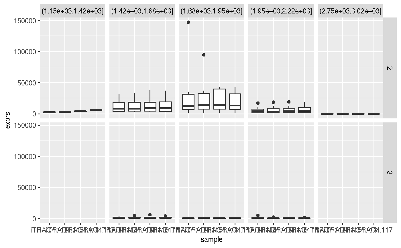
Future work
See issues, and the TODO issue in particular for current and future work. Depending on interest, the functionality presented here could be extended to other data types such as SummarizedExperiments.
A technical issue is with the dependency on both Bioconductor and the tidyverse is the recurrent name clashes:
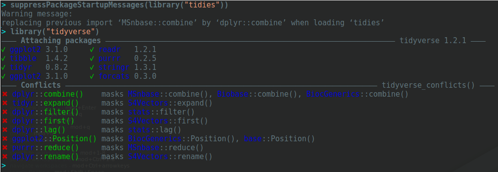
Bioconductor and tidyverse conflicts
The combine function, for example, is defined as a generic with signature combine(x, y, ...) in BiocGenerics, while it is combine(...) in dplyr.