MSnbase benchmarking • MSnbase

Introduction

In this vignette, we will document various timings and benchmarkings of the MSnbase version 2, that focuses on on-disk data access (as opposed to in-memory). More details about the new implementation are documented in the respective classes manual pages and in

MSnbase, efficient and elegant R-based processing and visualisation of raw mass spectrometry data. Laurent Gatto, Sebastian Gibb, Johannes Rainer. bioRxiv 2020.04.29.067868; doi: https://doi.org/10.1101/2020.04.29.067868

As a benchmarking dataset, we are going to use a subset of an TMT 6-plex experiment acquired on an LTQ Orbitrap Velos, that is distributed with the MsDataHub package

library("MsDataHub")

## Registered S3 method overwritten by 'bit64':
##   method          from 
##   print.bitstring tools

f <- TMT_Erwinia_1uLSike_Top10HCD_isol2_45stepped_60min_01.20141210.mzML.gz()

## see ?MsDataHub and browseVignettes('MsDataHub') for documentation

## loading from cache

We need to load the MSnbase package and set the session-wide verbosity flag to FALSE.

library("MSnbase")
setMSnbaseVerbose(FALSE)

Benchmarking

Reading data

We first read the data using the original behaviour readMSData function by setting the mode argument to "inMemory" to generates an in-memory representation of the MS2-level raw data and measure the time needed for this operation.

system.time(inmem <- readMSData(f, msLevel. = 2,
                                mode = "inMemory",
                                centroided. = TRUE))

##    user  system elapsed 
##  42.742   0.734  43.011

Next, we use the readMSData function to generate an on-disk representation of the same data by setting mode = "onDisk".

system.time(ondisk <- readMSData(f, msLevel. = 2,
                                  mode = "onDisk",
                                  centroided. = TRUE))

##    user  system elapsed 
##   8.881   0.504   8.932

Creating the on-disk experiment is considerable faster and scales to much bigger, multi-file data, both in terms of object creation time, but also in terms of object size (see next section). We must of course make sure that these two datasets are equivalent:

all.equal(inmem, ondisk)

## [1] TRUE

Data size

To compare the size occupied in memory of these two objects, we are going to use the object.size function, which accounts for the data (the spectra) in the assayData environment (as opposed to the object.size function from the utils package).

print(object.size(inmem), units = "MiB")

## 0.5 MiB

print(object.size(ondisk), units = "MiB")

## 2.8 MiB

The difference is explained by the fact that for ondisk, the spectra are not created and stored in memory; they are access on disk when needed, such as for example for plotting:

plot(inmem[[200]], full = TRUE)
plot(ondisk[[200]], full = TRUE)

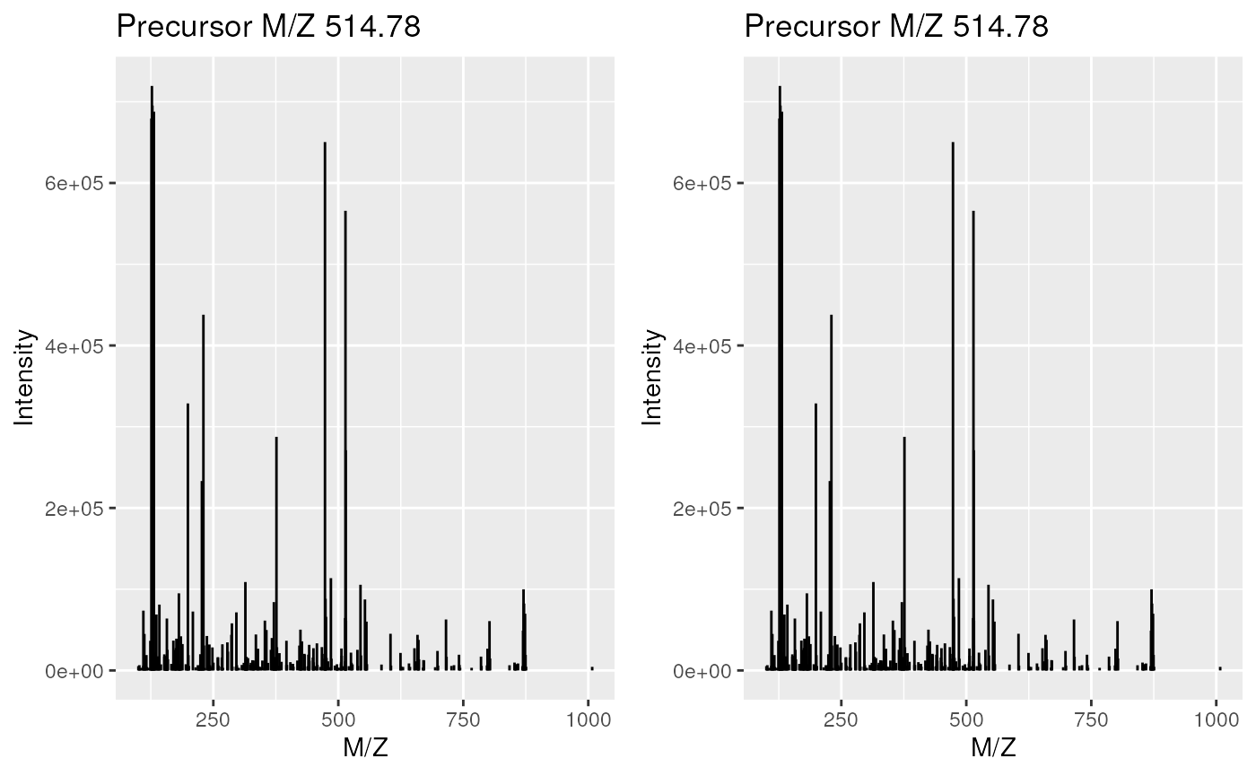
Plotting in-memory and on-disk spectra

Accessing spectra

The drawback of the on-disk representation is when the spectrum data has to actually be accessed. To compare access time, we are going to use the microbenchmark and repeat access 10 times to compare access to all 6103 and a single spectrum in-memory (i.e. pre-loaded and constructed) and on-disk (i.e. on-the-fly access).

library("microbenchmark")
mb <- microbenchmark(spectra(inmem),
                     inmem[[200]],
                     spectra(ondisk),
                     ondisk[[200]],
                     times = 10)
mb

## Unit: microseconds
##             expr         min          lq         mean      median          uq
##   spectra(inmem)    1089.585    1314.865    2436.7329    2792.699    3175.118
##     inmem[[200]]      24.897      26.380      70.1502      75.406     104.595
##  spectra(ondisk) 3827662.695 3855243.965 4703240.8731 3939344.255 5648236.757
##    ondisk[[200]] 1457927.203 1460082.357 1469420.5563 1472979.672 1474746.619
##          max neval
##     3237.906    10
##      143.839    10
##  6801170.483    10
##  1481629.040    10

While it takes order or magnitudes more time to access the data on-the-fly rather than a pre-generated spectrum, accessing all spectra is only marginally slower than accessing all spectra, as most of the time is spent preparing the file for access, which is done only once.

On-disk access performance will depend on the read throughput of the disk. A comparison of the data import of the above file from an internal solid state drive and from an USB3 connected hard disk showed only small differences for the onDisk mode (1.07 vs 1.36 seconds), while no difference were observed for accessing individual or all spectra. Thus, for this particular setup, performance was about the same for SSD and HDD. This might however not apply to setting in which data import is performed in parallel from multiple files.

Data access does not prohibit interactive usage, such as plotting, for example, as it is about 1/2 seconds, which is an operation that is relatively rare, compared to subsetting and filtering, which are faster for on-disk data:

i <- sample(length(inmem), 100)
system.time(inmem[i])

##    user  system elapsed 
##   0.140   0.000   0.139

system.time(ondisk[i])

##    user  system elapsed 
##   0.011   0.000   0.011

Operations on the spectra data, such as peak picking, smoothing, cleaning, … are cleverly cached and only applied when the data is accessed, to minimise file access overhead. Finally, specific operations such as for example quantitation (see next section) are optimised for speed.

MS2 quantitation

Below, we perform TMT 6-plex reporter ions quantitation on the first 100 spectra and verify that the results are identical (ignoring feature names).

system.time(eim <- quantify(inmem[1:100], reporters = TMT6,
                            method = "max"))

##    user  system elapsed 
##   3.653   1.677   1.549

system.time(eod <- quantify(ondisk[1:100], reporters = TMT6,
                            method = "max"))

##    user  system elapsed 
##   1.532   0.346   1.672

all.equal(eim, eod, check.attributes = FALSE)

## [1] TRUE

Notable differences on-disk and in-memory implementations

The MSnExp and OnDiskMSnExp documentation files and the MSnbase developement vignette provide more information about implementation details.

MS levels

On-disk support multiple MS levels in one object, while in-memory only supports a single level. While support for multiple MS levels could be added to the in-memory back-end, memory constrains make this pretty-much useless and will most likely never happen.

Serialisation

In-memory objects can be save()ed and load()ed, while on-disk can’t. As a workaround, the latter can be coerced to in-memory instances with as(, "MSnExp"). We would need mzML write support in mzR to be able to implement serialisation for on-disk data.

Data processing

Whenever possible, accessing and processing on-disk data is delayed (lazy processing). These operations are stored in a processing queue until the spectra are effectively instantiated.

Validity

The on-disk validObject method doesn’t verify the validity on the spectra (as there aren’t any to check). The validateOnDiskMSnExp function, on the other hand, instantiates all spectra and checks their validity (in addition to calling validObject).

Conclusions

This document focuses on speed and size improvements of the new on-disk MSnExp representation. The extend of these improvements will substantially increase for larger data.

For general functionality about the on-disk MSnExp data class and MSnbase in general, see other vignettes available with

vignette(package = "MSnbase")