MSnbase IO capabilities
Laurent Gatto
de Duve Institute, UCLouvain, BelgiumSource:
vignettes/v02-MSnbase-io.Rmd
v02-MSnbase-io.RmdAbstract
This vignette describes MSnbase’s input and output capabilities.
Foreword
This software is free and open-source software. If you use it, please support the project by citing it in publications:
Gatto L, Lilley KS. MSnbase-an R/Bioconductor package for isobaric tagged mass spectrometry data visualization, processing and quantitation. Bioinformatics. 2012 Jan 15;28(2):288-9. doi: 10.1093/bioinformatics/btr645. PMID: 22113085.
MSnbase, efficient and elegant R-based processing and visualisation of raw mass spectrometry data. Laurent Gatto, Sebastian Gibb, Johannes Rainer. bioRxiv 2020.04.29.067868; doi: https://doi.org/10.1101/2020.04.29.067868
Questions and bugs
For bugs, typos, suggestions or other questions, please file an issue
in our tracking system (https://github.com/lgatto/MSnbase/issues) providing as
much information as possible, a reproducible example and the output of
sessionInfo().
If you don’t have a GitHub account or wish to reach a broader audience for general questions about proteomics analysis using R, you may want to use the Bioconductor support site: https://support.bioconductor.org/.
Overview
MSnbase’s aims are to facilitate the reproducible analysis of mass spectrometry data within the R environment, from raw data import and processing, feature quantification, quantification and statistical analysis of the results (Gatto and Lilley 2012). Data import functions for several formats are provided and intermediate or final results can also be saved or exported. These capabilities are presented below.
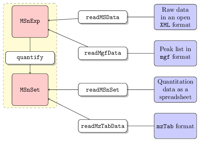
Data input
Raw data
Data stored in one of the published XML-based formats.
i.e. mzXML (Pedrioli et al.
2004), mzData (Orchard et al.
2007) or mzML (Martens et al.
2010), can be imported with the readMSData method,
which makes use of the mzR package
to create MSnExp objects. The files can be in profile or
centroided mode. See ?readMSData for details.
Data from mzML files containing chromatographic data
(e.g. generated in SRM/MRM experiments) can be imported with the
readSRMData function that returns the chromatographic data
as a MChromatograms object. See ?readSRMData
for more details.
Peak lists
Peak lists in the mgf format1 can be imported using
the readMgfData. In this case, the peak data has generally
been pre-processed by other software. See ?readMgfData for
details.
Quantitation data
Third party software can be used to generate quantitative data and
exported as a spreadsheet (generally comma or tab separated format).
This data as well as any additional meta-data can be imported with the
readMSnSet function. See ?readMSnSet for
details.
MSnbase
also supports the mzTab format2, a light-weight,
tab-delimited file format for proteomics data developed within the
Proteomics Standards Initiative (PSI). mzTab files can be
read into R with readMzTabData to create and
MSnSet instance.
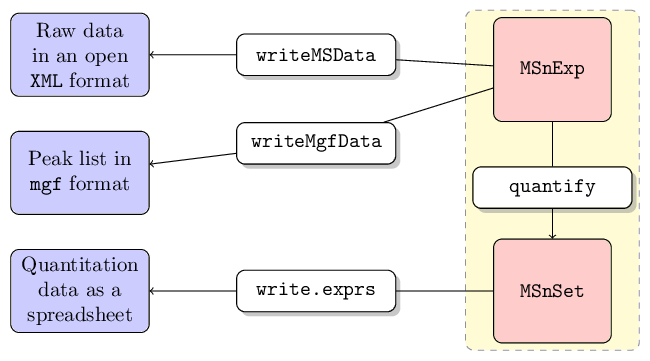
Data output
RData files
R objects can most easily be stored on disk with the
save function. It creates compressed binary images of the
data representation that can later be read back from the file with the
load function.
mzML/mzXML files
MSnExp and OnDiskMSnExp files can be
written to MS data files in mzML or mzXML
files with the writeMSData method. See
?writeMSData for details.
Peak lists
MSnExp instances as well as individual spectra can be
written as mgf files with the writeMgfData
method. Note that the meta-data in the original R object can not be
included in the file. See ?writeMgfData for details.
Quantitation data
Quantitation data can be exported to spreadsheet files with the
write.exprs method. Feature meta-data can be appended to
the feature intensity values. See ?writeMgfData for
details.
Deprecated MSnSet instances can also be
exported to mzTab files using the
writeMzTabData function.
Creating MSnSet from text spread sheets
This section describes the generation of MSnSet objects
using data available in a text-based spreadsheet. This entry point into
R and MSnbase
allows to import data processed by any of the third party
mass-spectrometry processing software available and proceed with data
exploration, normalisation and statistical analysis using functions
available in and the numerous Bioconductor packages.
A complete work flow
The following section describes a work flow that uses three input
files to create the MSnSet. These files respectively
describe the quantitative expression data, the sample meta-data and the
feature meta-data. It is taken from the pRoloc
tutorial and uses example files from the pRolocdat
package.
We start by describing the csv to be used as input using
the read.csv function.
## The original data for replicate 1, available
## from the pRolocdata package
f0 <- dir(system.file("extdata", package = "pRolocdata"),
          full.names = TRUE,
          pattern = "pr800866n_si_004-rep1.csv")
csv <- read.csv(f0)
The three first lines of the original spreadsheet, containing the
data for replicate one, are illustrated below (using the function
head). It contains 888 rows (proteins) and 16 columns,
including protein identifiers, database accession numbers, gene symbols,
reporter ion quantitation values, information related to protein
identification, …
head(csv, n=3)## Protein.ID FBgn Flybase.Symbol No..peptide.IDs Mascot.score
## 1 CG10060 FBgn0001104 G-ialpha65A 3 179.86
## 2 CG10067 FBgn0000044 Act57B 5 222.40
## 3 CG10077 FBgn0035720 CG10077 5 219.65
## No..peptides.quantified area.114 area.115 area.116 area.117
## 1 1 0.379000 0.281000 0.225000 0.114000
## 2 9 0.420000 0.209667 0.206111 0.163889
## 3 3 0.187333 0.167333 0.169667 0.476000
## PLS.DA.classification Peptide.sequence Precursor.ion.mass
## 1 PM
## 2 PM
## 3
## Precursor.ion.charge pd.2013 pd.markers
## 1 PM unknown
## 2 PM unknown
## 3 unknown unknownBelow read in turn the spread sheets that contain the quantitation
data (exprsFile.csv), feature meta-data
(fdataFile.csv) and sample meta-data
(pdataFile.csv).
## The quantitation data, from the original data
f1 <- dir(system.file("extdata", package = "pRolocdata"),
          full.names = TRUE, pattern = "exprsFile.csv")
exprsCsv <- read.csv(f1)
## Feature meta-data, from the original data
f2 <- dir(system.file("extdata", package = "pRolocdata"),
          full.names = TRUE, pattern = "fdataFile.csv")
fdataCsv <- read.csv(f2)
## Sample meta-data, a new file
f3 <- dir(system.file("extdata", package = "pRolocdata"),
          full.names = TRUE, pattern = "pdataFile.csv")
pdataCsv <- read.csv(f3)
exprsFile.csv contains the quantitation (expression)
data for the 888 proteins and 4 reporter tags.
head(exprsCsv, n = 3)## FBgn X114 X115 X116 X117
## 1 FBgn0001104 0.379000 0.281000 0.225000 0.114000
## 2 FBgn0000044 0.420000 0.209667 0.206111 0.163889
## 3 FBgn0035720 0.187333 0.167333 0.169667 0.476000fdataFile.csv contains meta-data for the 888 features
(here proteins).
head(fdataCsv, n = 3)## FBgn ProteinID FlybaseSymbol NoPeptideIDs MascotScore
## 1 FBgn0001104 CG10060 G-ialpha65A 3 179.86
## 2 FBgn0000044 CG10067 Act57B 5 222.40
## 3 FBgn0035720 CG10077 CG10077 5 219.65
## NoPeptidesQuantified PLSDA
## 1 1 PM
## 2 9 PM
## 3 3pdataFile.csv contains samples (here fractions)
meta-data. This simple file has been created manually.
pdataCsv## sampleNames Fractions
## 1 X114 4/5
## 2 X115 12/13
## 3 X116 19
## 4 X117 21The self-contained MSnSet can now easily be generated
using the readMSnSet constructor, providing the respective
csv file names shown above and specifying that the data is
comma-separated (with sep = ","). Below, we call that
object res and display its content.
library("MSnbase")
res <- readMSnSet(exprsFile = f1,
                  featureDataFile = f2,
                  phenoDataFile = f3,
                  sep = ",")
res
## MSnSet (storageMode: lockedEnvironment)
## assayData: 888 features, 4 samples
## element names: exprs
## protocolData: none
## phenoData
## sampleNames: X114 X115 X116 X117
## varLabels: Fractions
## varMetadata: labelDescription
## featureData
## featureNames: FBgn0001104 FBgn0000044 ... FBgn0001215 (888 total)
## fvarLabels: ProteinID FlybaseSymbol ... PLSDA (6 total)
## fvarMetadata: labelDescription
## experimentData: use 'experimentData(object)'
## Annotation:
## - - - Processing information - - -
## Quantitation data loaded: Wed Jul 8 15:21:17 2026 using readMSnSet.
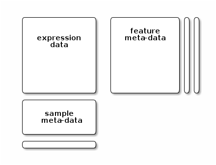
## MSnbase version: 2.39.2The MSnSet class
Although there are additional specific sub-containers for additional
meta-data (for instance to make the object MIAPE compliant), the feature
(the sub-container, or slot featureData) and sample (the
phenoData slot) are the most important ones. They need to
meet the following validity requirements (see figure below):
the number of row in the expression/quantitation data and feature data must be equal and the row names must match exactly, and
the number of columns in the expression/quantitation data and number of row in the sample meta-data must be equal and the column/row names must match exactly.
A detailed description of the MSnSet class is available
by typing ?MSnSet in the R console.
The individual parts of this data object can be accessed with their respective accessor methods:
- the quantitation data can be retrieved with
exprs(res), - the feature meta-data with
fData(res)and - the sample meta-data with
pData(res).
A shorter work flow
The readMSnSet2 function provides a simplified import
workforce. It takes a single spreadsheet as input (default is
csv) and extract the columns identified by
ecol to create the expression data, while the others are
used as feature meta-data. ecol can be a
character with the respective column labels or a numeric
with their indices. In the former case, it is important to make sure
that the names match exactly. Special characters like '-'
or '(' will be transformed by R into '.' when
the csv file is read in. Optionally, one can also specify a
column to be used as feature names. Note that these must be unique to
guarantee the final object validity.
ecol <- paste("area", 114:117, sep = ".")
fname <- "Protein.ID"
eset <- readMSnSet2(f0, ecol, fname)
eset
## MSnSet (storageMode: lockedEnvironment)
## assayData: 888 features, 4 samples
## element names: exprs
## protocolData: none
## phenoData: none
## featureData
## featureNames: CG10060 CG10067 ... CG9983 (888 total)
## fvarLabels: Protein.ID FBgn ... pd.markers (12 total)
## fvarMetadata: labelDescription
## experimentData: use 'experimentData(object)'
## Annotation:
## - - - Processing information - - -
## MSnbase version: 2.39.2The ecol columns can also be queried interactively from
R using the getEcols and grepEcols function.
The former return a character with all column names, given a splitting
character, i.e. the separation value of the spreadsheet (typically
"," for csv, "\t" for
tsv, …). The latter can be used to grep a pattern of
interest to obtain the relevant column indices.
getEcols(f0, ",")## [1] "\"Protein ID\"" "\"FBgn\""
## [3] "\"Flybase Symbol\"" "\"No. peptide IDs\""
## [5] "\"Mascot score\"" "\"No. peptides quantified\""
## [7] "\"area 114\"" "\"area 115\""
## [9] "\"area 116\"" "\"area 117\""
## [11] "\"PLS-DA classification\"" "\"Peptide sequence\""
## [13] "\"Precursor ion mass\"" "\"Precursor ion charge\""
## [15] "\"pd.2013\"" "\"pd.markers\""
grepEcols(f0, "area", ",")## [1] 7 8 9 10
e <- grepEcols(f0, "area", ",")
readMSnSet2(f0, e)
## MSnSet (storageMode: lockedEnvironment)
## assayData: 888 features, 4 samples
## element names: exprs
## protocolData: none
## phenoData: none
## featureData
## featureNames: 1 2 ... 888 (888 total)
## fvarLabels: Protein.ID FBgn ... pd.markers (12 total)
## fvarMetadata: labelDescription
## experimentData: use 'experimentData(object)'
## Annotation:
## - - - Processing information - - -
## MSnbase version: 2.39.2The phenoData slot can now be updated accordingly using
the replacement functions phenoData<- or
pData<- (see ?MSnSet for details).
Session information
## R version 4.6.1 (2026-06-24)
## Platform: x86_64-pc-linux-gnu
## Running under: Ubuntu 24.04.4 LTS
##
## Matrix products: default
## BLAS:   /usr/lib/x86_64-linux-gnu/openblas-pthread/libblas.so.3
## LAPACK: /usr/lib/x86_64-linux-gnu/openblas-pthread/libopenblasp-r0.3.26.so;  LAPACK version 3.12.0
##
## locale:
##  [1] LC_CTYPE=en_US.UTF-8       LC_NUMERIC=C
##  [3] LC_TIME=en_US.UTF-8        LC_COLLATE=en_US.UTF-8
##  [5] LC_MONETARY=en_US.UTF-8    LC_MESSAGES=en_US.UTF-8
##  [7] LC_PAPER=en_US.UTF-8       LC_NAME=C
##  [9] LC_ADDRESS=C               LC_TELEPHONE=C
## [11] LC_MEASUREMENT=en_US.UTF-8 LC_IDENTIFICATION=C
##
## time zone: UTC
## tzcode source: system (glibc)
##
## attached base packages:
## [1] stats4    stats     graphics  grDevices utils     datasets  methods
## [8] base
##
## other attached packages:
##  [1] pRolocdata_1.50.0   MSnbase_2.39.2      ProtGenerics_1.44.0
##  [4] S4Vectors_0.50.1    mzR_2.46.0          Rcpp_1.1.2
##  [7] Biobase_2.72.0      BiocGenerics_0.58.1 generics_0.1.4
## [10] BiocStyle_2.40.0
##
## loaded via a namespace (and not attached):
##  [1] rlang_1.3.0                 magrittr_2.0.5
##  [3] clue_0.3-68                 otel_0.2.0
##  [5] matrixStats_1.5.0           compiler_4.6.1
##  [7] PTMods_1.1.1                systemfonts_1.3.2
##  [9] vctrs_0.7.3                 reshape2_1.4.5
## [11] stringr_1.6.0               pkgconfig_2.0.3
## [13] MetaboCoreUtils_1.20.1      fastmap_1.2.0
## [15] XVector_0.52.0              rmarkdown_2.31
## [17] preprocessCore_1.75.0       ragg_1.5.2
## [19] purrr_1.2.2                 xfun_0.59
## [21] MultiAssayExperiment_1.38.0 cachem_1.1.0
## [23] jsonlite_2.0.0              DelayedArray_0.38.2
## [25] BiocParallel_1.46.0         parallel_4.6.1
## [27] cluster_2.1.8.2             R6_2.6.1
## [29] bslib_0.11.0                stringi_1.8.7
## [31] RColorBrewer_1.1-3          limma_3.68.4
## [33] GenomicRanges_1.64.0        jquerylib_0.1.4
## [35] iterators_1.0.14            Seqinfo_1.2.0
## [37] bookdown_0.47               SummarizedExperiment_1.42.0
## [39] knitr_1.51                  IRanges_2.46.0
## [41] Matrix_1.7-5                igraph_2.3.3
## [43] tidyselect_1.2.1            abind_1.4-8
## [45] yaml_2.3.12                 doParallel_1.0.17
## [47] codetools_0.2-20            affy_1.90.0
## [49] lattice_0.22-9              tibble_3.3.1
## [51] plyr_1.8.9                  S7_0.2.2
## [53] evaluate_1.0.5              desc_1.4.3
## [55] Spectra_1.22.2              pillar_1.11.1
## [57] affyio_1.82.0               BiocManager_1.30.27
## [59] MatrixGenerics_1.24.0       foreach_1.5.2
## [61] MALDIquant_1.22.3           ncdf4_1.24
## [63] ggplot2_4.0.3               scales_1.4.0
## [65] glue_1.8.1                  lazyeval_0.2.3
## [67] tools_4.6.1                 mzID_1.50.0
## [69] data.table_1.18.4           QFeatures_1.22.0
## [71] vsn_3.80.0                  fs_2.1.0
## [73] XML_3.99-0.23               grid_4.6.1
## [75] impute_1.86.0               tidyr_1.3.2
## [77] MsCoreUtils_1.24.0          PSMatch_1.17.1
## [79] cli_3.6.6                   textshaping_1.0.5
## [81] S4Arrays_1.12.0             dplyr_1.2.1
## [83] AnnotationFilter_1.36.0     pcaMethods_2.4.0
## [85] gtable_0.3.6                sass_0.4.10
## [87] digest_0.6.39               SparseArray_1.12.2
## [89] htmlwidgets_1.6.4           farver_2.1.2
## [91] htmltools_0.5.9             pkgdown_2.2.1.9000
## [93] lifecycle_1.0.5             statmod_1.5.2
## [95] MASS_7.3-65