Last modified: NA
Compiled: Thu Aug 12 15:59:13 2021

Introduction

QFeatures is a package for the manipulation of mass spectrometry (MS)-based quantitative proteomics data. The quantitative data is generally obtained after running a preprocessing algorithm on raw MS profiles called spectra. The algorithm attempts to match each spectra to a peptide database to infer the peptide sequence. A spectrum for which a corresponding peptide could be found is called peptide to spectrum match (PSM). The intensities recorded by the MS are then used to quantify the PSMs. The quantified PSMs are used as input by QFeatures and undergo various data wrangling steps to reconstruct the peptide data and then the protein data, usually of interest for elucidating the biological question at hand.

MS-based quantification data can be represented as a matrix of quantitative values for features (PSMs, peptides, proteins) arranged along the rows, measured for a set of samples, arranged along the columns. The matrix format is a common representation for any quantitative data set. We will be using the SummarizedExperiment (Morgan et al. 2020) class:

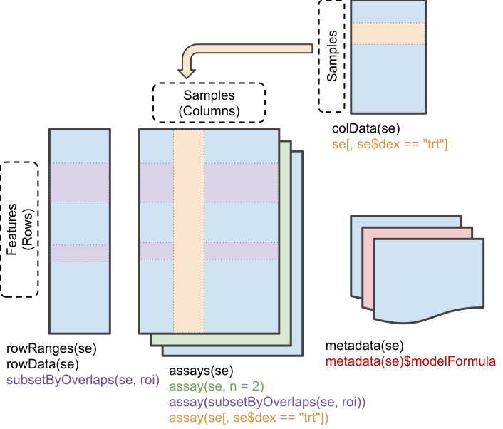
Schematic representation of the anatomy of a SummarizedExperiment object. (Figure taken from the SummarizedExperiment package vignette.)

The sample (columns) metadata can be access with the colData() function.
The features (rows) metadata can be access with the rowData() column.
The quantiative data can be accessed with assay().
assays() returns a list of matrix-like assays.

Note that other classes that inherits from SummarizedExperiment can also be used. We will see in the other vignette that for single-cell proteomics data, we will use SingleCellExperiment objects.

QFeatures

While mass spectrometers acquire data for spectra/peptides, the biological entity of interest are the protein. As part of the data processing, we are thus required to aggregate low-level quantitative features into higher level data.

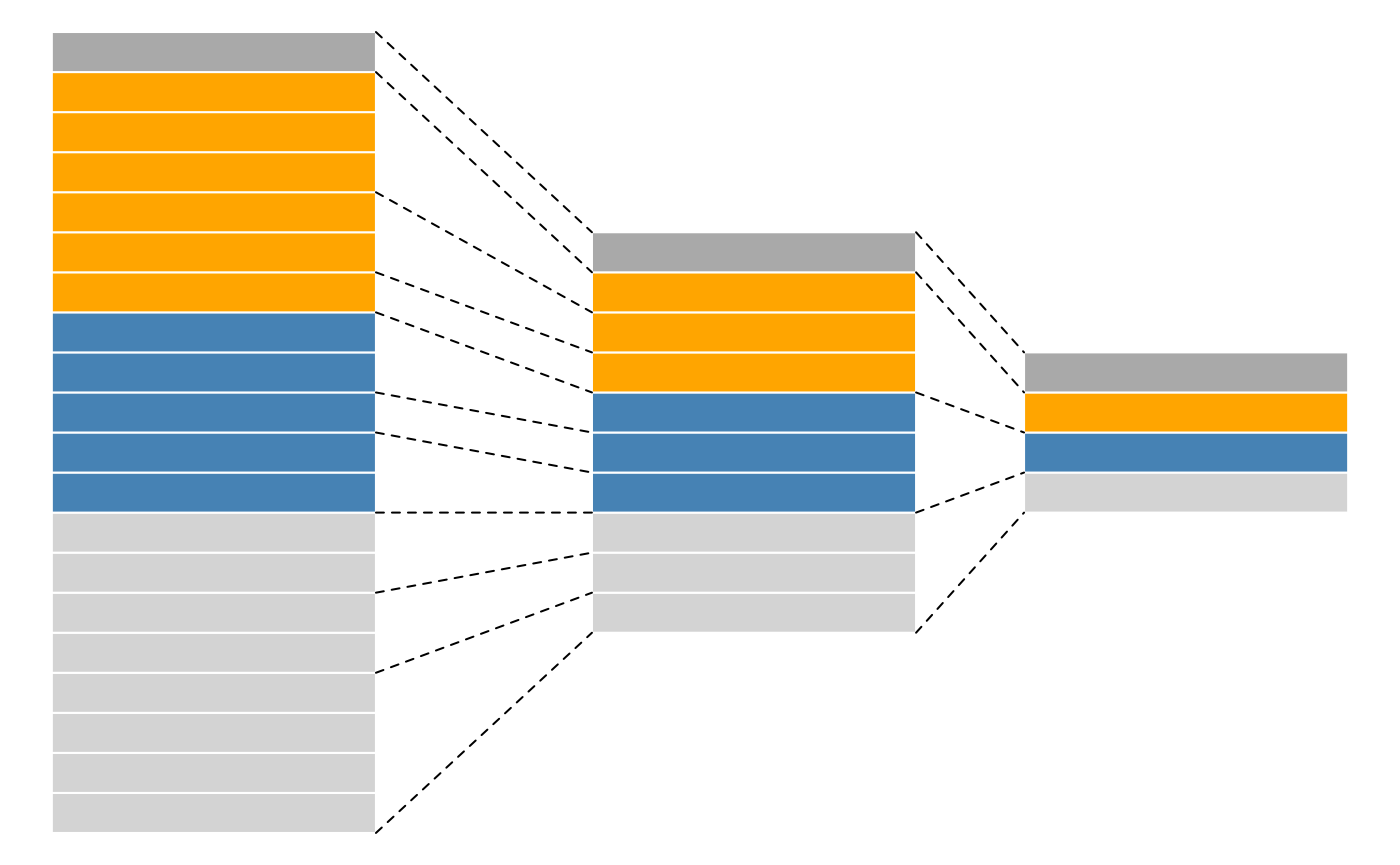
Conceptual representation of a QFeatures object and the aggregative relation between different assays.

We are going to start to familiarise ourselves with the QFeatures class implemented in the QFeatures package. The class is derived from the Bioconductor MultiAssayExperiment (Ramos et al. 2017) class. Let’s start by loading the QFeatures package.

library("QFeatures")

Next, we load the feat1 test data, which is composed of single assay of class SummarizedExperiment composed of 10 rows and 2 columns.

data(feat1)
feat1
## An instance of class QFeatures containing 1 assays:
##  [1] psms: SummarizedExperiment with 10 rows and 2 columns

Let’s perform some simple operations to familiarise ourselves with the QFeatures class:

Extract the sample metadata using the colData() accessor (like you have previously done with SummarizedExperiment objects).

colData(feat1)
## DataFrame with 2 rows and 1 column
##        Group
##    <integer>
## S1         1
## S2         2

Extract the first (and only) assay composing this QFeaures data using the [[ operator (as you have done to extract elements of a list) by using the assay’s index or name.

feat1[[1]]
## class: SummarizedExperiment 
## dim: 10 2 
## metadata(0):
## assays(1): ''
## rownames(10): PSM1 PSM2 ... PSM9 PSM10
## rowData names(5): Sequence Protein Var location pval
## colnames(2): S1 S2
## colData names(0):
feat1[["psms"]]
## class: SummarizedExperiment 
## dim: 10 2 
## metadata(0):
## assays(1): ''
## rownames(10): PSM1 PSM2 ... PSM9 PSM10
## rowData names(5): Sequence Protein Var location pval
## colnames(2): S1 S2
## colData names(0):

Extract the psms assay’s row data and quantitative values.

assay(feat1[[1]])
##       S1 S2
## PSM1   1 11
## PSM2   2 12
## PSM3   3 13
## PSM4   4 14
## PSM5   5 15
## PSM6   6 16
## PSM7   7 17
## PSM8   8 18
## PSM9   9 19
## PSM10 10 20
rowData(feat1[[1]])
## DataFrame with 10 rows and 5 columns
##            Sequence     Protein       Var      location      pval
##         <character> <character> <integer>   <character> <numeric>
## PSM1       SYGFNAAR       ProtA         1 Mitochondr...     0.084
## PSM2       SYGFNAAR       ProtA         2 Mitochondr...     0.077
## PSM3       SYGFNAAR       ProtA         3 Mitochondr...     0.063
## PSM4       ELGNDAYK       ProtA         4 Mitochondr...     0.073
## PSM5       ELGNDAYK       ProtA         5 Mitochondr...     0.012
## PSM6       ELGNDAYK       ProtA         6 Mitochondr...     0.011
## PSM7  IAEESNFPFI...       ProtB         7       unknown     0.075
## PSM8  IAEESNFPFI...       ProtB         8       unknown     0.038
## PSM9  IAEESNFPFI...       ProtB         9       unknown     0.028
## PSM10 IAEESNFPFI...       ProtB        10       unknown     0.097

Feature aggregation

The central functionality of the QFeatures infrastructure is the aggregation of features into higher-level features while retaining the link between the different levels. This can be done with the aggregateFeatures() function.

The call below will

operate on the psms assay of the feat1 objects;
aggregate the rows the assay following the grouping defined in the peptides row data variables;
perform aggregation using the colMeans() function;
create a new assay named peptides and add it to the feat1 object.

feat1 <- aggregateFeatures(feat1, i = "psms",
                           fcol = "Sequence",
                           name = "peptides",
                           fun = colMeans)
feat1
## An instance of class QFeatures containing 2 assays:
##  [1] psms: SummarizedExperiment with 10 rows and 2 columns 
##  [2] peptides: SummarizedExperiment with 3 rows and 2 columns

Note: we do not claim that colMeans is the best aggregation method. There are other more robust methods for aggregating features, for instance MsCoreUtils::robustSummary is a good alternative. See the documentation of aggregateFeatures for more information.

Exercise at home: check that you understand the effect of feature aggregation and repeat the calculations manually. Compare your manual results agains the content of the new assay’s row data.

Solution

## Data before aggregation
data.frame(assay(feat1[["psms"]]), 
           Sequence = rowData(feat1[["psms"]])$Sequence)
##       S1 S2    Sequence
## PSM1   1 11    SYGFNAAR
## PSM2   2 12    SYGFNAAR
## PSM3   3 13    SYGFNAAR
## PSM4   4 14    ELGNDAYK
## PSM5   5 15    ELGNDAYK
## PSM6   6 16    ELGNDAYK
## PSM7   7 17 IAEESNFPFIK
## PSM8   8 18 IAEESNFPFIK
## PSM9   9 19 IAEESNFPFIK
## PSM10 10 20 IAEESNFPFIK

## SYGFNAAR
colMeans(assay(feat1[["psms"]])[1:3, ])
## S1 S2 
##  2 12
assay(feat1[[2]])["SYGFNAAR", ]
## S1 S2 
##  2 12

## ELGNDAYK
colMeans(assay(feat1[["psms"]])[4:6, ])
## S1 S2 
##  5 15
assay(feat1[[2]])["ELGNDAYK", ]
## S1 S2 
##  5 15

## IAEESNFPFIK
colMeans(assay(feat1[["psms"]])[7:10, ])
##   S1   S2 
##  8.5 18.5
assay(feat1[[2]])["IAEESNFPFIK", ]
##   S1   S2 
##  8.5 18.5

rowData(feat1[[2]])
## DataFrame with 3 rows and 4 columns
##                  Sequence     Protein      location        .n
##               <character> <character>   <character> <integer>
## ELGNDAYK         ELGNDAYK       ProtA Mitochondr...         3
## IAEESNFPFIK IAEESNFPFI...       ProtB       unknown         4
## SYGFNAAR         SYGFNAAR       ProtA Mitochondr...         3

We can now aggregate the peptide-level data into a new protein-level assay using the colMedians() aggregation function.

feat1 <- aggregateFeatures(feat1, i = "peptides",
                           fcol = "Protein",
                           name = "proteins",
                           fun = colMedians)
feat1
## An instance of class QFeatures containing 3 assays:
##  [1] psms: SummarizedExperiment with 10 rows and 2 columns 
##  [2] peptides: SummarizedExperiment with 3 rows and 2 columns 
##  [3] proteins: SummarizedExperiment with 2 rows and 2 columns
assay(feat1[["proteins"]])
##        S1   S2
## ProtA 3.5 13.5
## ProtB 8.5 18.5

You can also get a graphical overview of the QFeatures object thanks to the plot function. Arrows represent the links between the assays.

plot(feat1)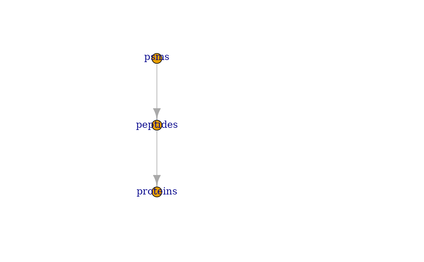

Subsetting and filtering

The subsetting a QFeatures object can be performed using the 3-index subset operator, [. The first index will subset the features of interest. If the feature is linked to features from other assays, those features will also

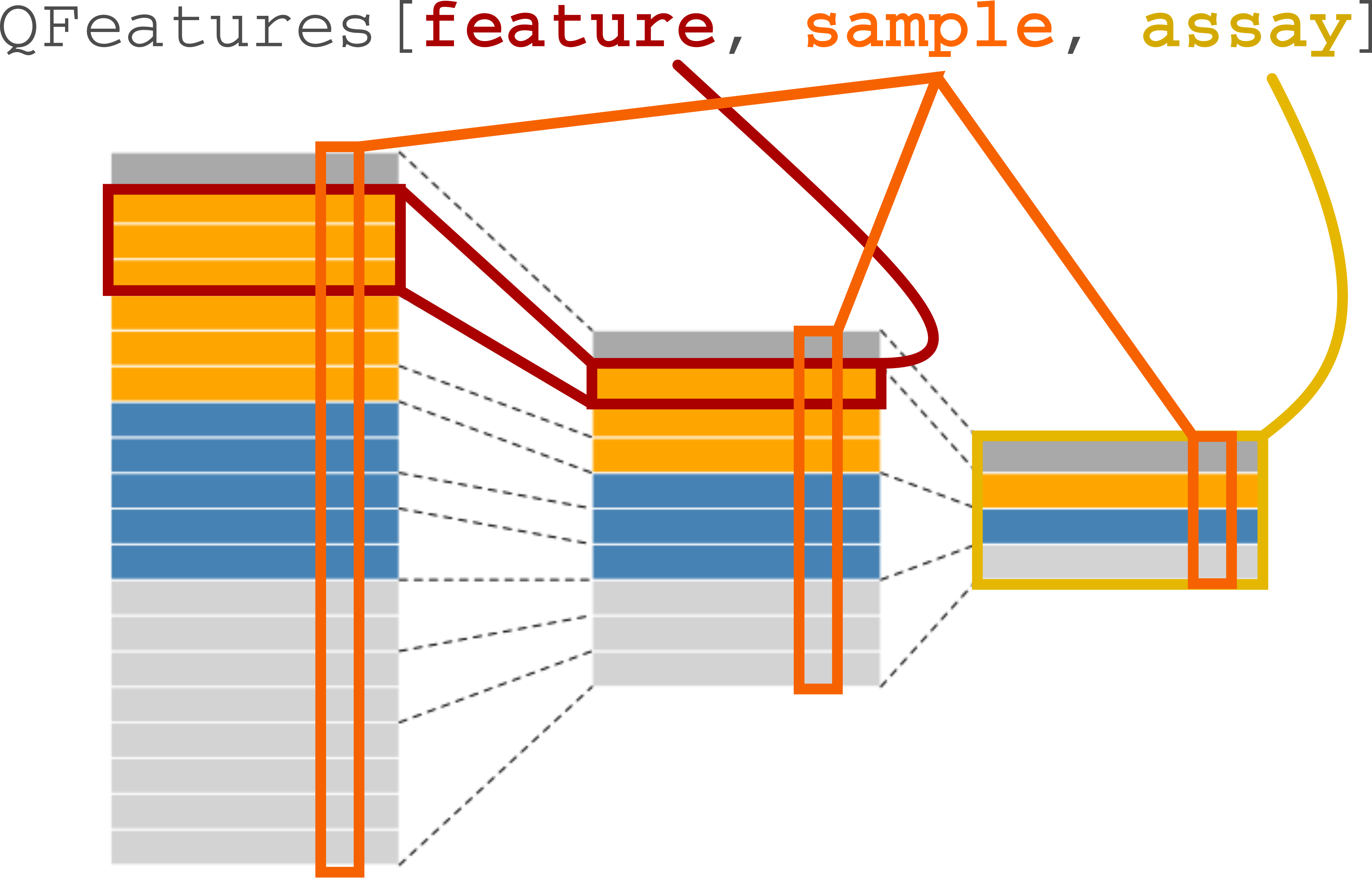
Conceptual illustration of the 3-index subsetting of QFeatures object.

We provide an example of subsetting features that are associated to features from other assays. When we subset for protein A as shown below or using the subsetByFeature() function, this creates a new instance of class QFeatures containing assays with the expression data for protein, its peptides and their PSMs.

feat1["ProtA", , ]
## An instance of class QFeatures containing 3 assays:
##  [1] psms: SummarizedExperiment with 6 rows and 2 columns 
##  [2] peptides: SummarizedExperiment with 2 rows and 2 columns 
##  [3] proteins: SummarizedExperiment with 1 rows and 2 columns

The filterFeatures() function can be used to filter rows the assays composing a QFeatures object using the row data variables. We can for example retain rows that have a pval < 0.05, which would only keep rows in the psms assay because the pval is only relevant for that assay.

filterFeatures(feat1, ~ pval < 0.05)
## An instance of class QFeatures containing 3 assays:
##  [1] psms: SummarizedExperiment with 4 rows and 2 columns 
##  [2] peptides: SummarizedExperiment with 0 rows and 2 columns 
##  [3] proteins: SummarizedExperiment with 0 rows and 2 columns

On the other hand, if we filter assay rows for those that localise to the mitochondrion, we retain the relevant protein, peptides and PSMs.

filterFeatures(feat1, ~ location == "Mitochondrion")
## An instance of class QFeatures containing 3 assays:
##  [1] psms: SummarizedExperiment with 6 rows and 2 columns 
##  [2] peptides: SummarizedExperiment with 2 rows and 2 columns 
##  [3] proteins: SummarizedExperiment with 1 rows and 2 columns

As an exercise, let’s filter rows that do not localise to the mitochondrion.

filterFeatures(feat1, ~ location != "Mitochondrion")
## An instance of class QFeatures containing 3 assays:
##  [1] psms: SummarizedExperiment with 4 rows and 2 columns 
##  [2] peptides: SummarizedExperiment with 1 rows and 2 columns 
##  [3] proteins: SummarizedExperiment with 1 rows and 2 columns

Another useful filtering functionality is filterNA that removes features based on the amount of missing data it contains. To illustrate this, we will load a data set containing missing data

data("ft_na")
ft_na
## An instance of class QFeatures containing 1 assays:
##  [1] na: SummarizedExperiment with 4 rows and 3 columns
assay(ft_na[[1]])
##    A  B  C
## a NA  5  9
## b  2  6 10
## c  3 NA 11
## d NA  8 12

We can remove feature that contain more that a given percentage missing values. For instance, let’s remove features with more than 25 % missing data. We expect to keep only 1 features as all the other features contain 33 % missing values.

filterNA(ft_na, i = "na", pNA = 0.25)
## An instance of class QFeatures containing 1 assays:
##  [1] na: SummarizedExperiment with 1 rows and 3 columns

The resulting QFeatures object contains a single feature as we expected.

Data processing

The Qfeatures package provides a few utility functions to process the data:

Logarithmic transform: logTransform creates a new assay in a QFeatures object that contains the log-transformed quantification of the target assay.

logTransform(feat1, i = "proteins", base = 2, name = "logproteins")
## An instance of class QFeatures containing 4 assays:
##  [1] psms: SummarizedExperiment with 10 rows and 2 columns 
##  [2] peptides: SummarizedExperiment with 3 rows and 2 columns 
##  [3] proteins: SummarizedExperiment with 2 rows and 2 columns 
##  [4] logproteins: SummarizedExperiment with 2 rows and 2 columns

Normalization: normalize creates a new assay in a QFeatures object that contains the normalized quantification of the target assay. See the ?QFeatures::normalize documentation for a list of available normalization methods. If the method you are looking for is not available, you could also consider QFeatures::sweep.

normalize(feat1, i = "proteins", method = "center.median", name = "normproteins")
## An instance of class QFeatures containing 4 assays:
##  [1] psms: SummarizedExperiment with 10 rows and 2 columns 
##  [2] peptides: SummarizedExperiment with 3 rows and 2 columns 
##  [3] proteins: SummarizedExperiment with 2 rows and 2 columns 
##  [4] normproteins: SummarizedExperiment with 2 rows and 2 columns

Imputation: imputes predicts missing values in a new assay. See the ?MsCoreUtils::impute_matrix() for a list of available imputation methods. In this example, we impute missing values with zero.

assay(ft_na[[1]])
##    A  B  C
## a NA  5  9
## b  2  6 10
## c  3 NA 11
## d NA  8 12
ft_na <- impute(ft_na, i = 1, method = "zero")
assay(ft_na[[1]])
##   A B  C
## a 0 5  9
## b 2 6 10
## c 3 0 11
## d 0 8 12

Session information

sessionInfo()
## R version 4.1.0 (2021-05-18)
## Platform: x86_64-pc-linux-gnu (64-bit)
## Running under: Ubuntu 20.04.2 LTS
## 
## Matrix products: default
## BLAS/LAPACK: /usr/lib/x86_64-linux-gnu/openblas-pthread/libopenblasp-r0.3.8.so
## 
## locale:
##  [1] LC_CTYPE=en_US.UTF-8       LC_NUMERIC=C              
##  [3] LC_TIME=en_US.UTF-8        LC_COLLATE=en_US.UTF-8    
##  [5] LC_MONETARY=en_US.UTF-8    LC_MESSAGES=C             
##  [7] LC_PAPER=en_US.UTF-8       LC_NAME=C                 
##  [9] LC_ADDRESS=C               LC_TELEPHONE=C            
## [11] LC_MEASUREMENT=en_US.UTF-8 LC_IDENTIFICATION=C       
## 
## attached base packages:
## [1] stats4    stats     graphics  grDevices utils     datasets  methods  
## [8] base     
## 
## other attached packages:
##  [1] QFeatures_1.3.7             MultiAssayExperiment_1.19.5
##  [3] SummarizedExperiment_1.23.1 Biobase_2.53.0             
##  [5] GenomicRanges_1.45.0        GenomeInfoDb_1.29.3        
##  [7] IRanges_2.27.0              S4Vectors_0.31.0           
##  [9] BiocGenerics_0.39.1         MatrixGenerics_1.5.3       
## [11] matrixStats_0.60.0          BiocStyle_2.21.3           
## 
## loaded via a namespace (and not attached):
##  [1] xfun_0.25               bslib_0.2.5.1           lattice_0.20-44        
##  [4] htmltools_0.5.1.1       yaml_2.2.1              rlang_0.4.11           
##  [7] pkgdown_1.6.1           jquerylib_0.1.4         GenomeInfoDbData_1.2.6 
## [10] stringr_1.4.0           zlibbioc_1.39.0         ProtGenerics_1.25.1    
## [13] ragg_1.1.3              memoise_2.0.0           evaluate_0.14          
## [16] knitr_1.33              fastmap_1.1.0           highr_0.9              
## [19] BiocManager_1.30.16     cachem_1.0.5            DelayedArray_0.19.1    
## [22] desc_1.3.0              jsonlite_1.7.2          XVector_0.33.0         
## [25] systemfonts_1.0.2       fs_1.5.0                MsCoreUtils_1.5.0      
## [28] textshaping_0.3.5       digest_0.6.27           stringi_1.7.3          
## [31] rprojroot_2.0.2         grid_4.1.0              clue_0.3-59            
## [34] tools_4.1.0             bitops_1.0-7            magrittr_2.0.1         
## [37] sass_0.4.0              RCurl_1.98-1.3          lazyeval_0.2.2         
## [40] cluster_2.1.2           pkgconfig_2.0.3         crayon_1.4.1           
## [43] MASS_7.3-54             Matrix_1.3-4            rmarkdown_2.10         
## [46] AnnotationFilter_1.17.1 R6_2.5.0                igraph_1.2.6           
## [49] compiler_4.1.0

References

Morgan, Martin, Valerie Obenchain, Jim Hester, and Hervé Pagès. 2020. SummarizedExperiment: SummarizedExperiment Container. https://bioconductor.org/packages/SummarizedExperiment.

Ramos, Marcel, Lucas Schiffer, Angela Re, Rimsha Azhar, Azfar Basunia, Carmen Rodriguez Cabrera, Tiffany Chan, et al. 2017. “Software for the Integration of Multi-Omics Experiments in Bioconductor.” Cancer Research 77(21); e39-42.

The QFeatures class

Laurent Gatto and Christophe Vanderaa