scp for single-cell proteomics analyses
Laurent Gatto and Christophe Vanderaa
Source:vignettes/v02-scp.Rmd
v02-scp.RmdLast modified: 2021-08-12 13:40:23
Compiled: Thu Aug 12 15:59:38 2021
Introduction
Mass spectrometry (MS)-based single-cell proteomics (SCP) is emerging thanks to several recent technological advances in sample preparation, liquid chromatography (LC) and MS (see Kelly (2020) for a comprehensive review). The improvements tackle the issues encountered when dealing with small sample amounts and focus on:
- Reducing sample loss
- Increasing sensitivity and quantification accuracy
- Increasing acquisition throughput
Two main strategies have currently been developed. On the one hand, label-free protocols acquire one single cell per MS run leading to accurate quantification but low sensitivity and throughput. On the other hand, label-based protocols multiplex several single-cell samples in one MS run leading to higher throughput (1000 cells per week). Another advantage of label-based protocols is the inclusion of a carrier sample, that is a sample containing between tens to hundreds of cells. Including a carrier increases sensitivity thanks to increased sample material, but at the cost of decreased quantification accuracy due to chemical noise (linked to sample labelling) and competition between the single-cell samples and the carrier sample during MS acquisition.
Although the scp package can handle the data acquired from the two strategies, the exercise of this vignette will focus on the multiplexed strategy developed by Specht et al. (2021), called SCoPE2. An overview of the acquisition and data processing pipeline is depicted below.
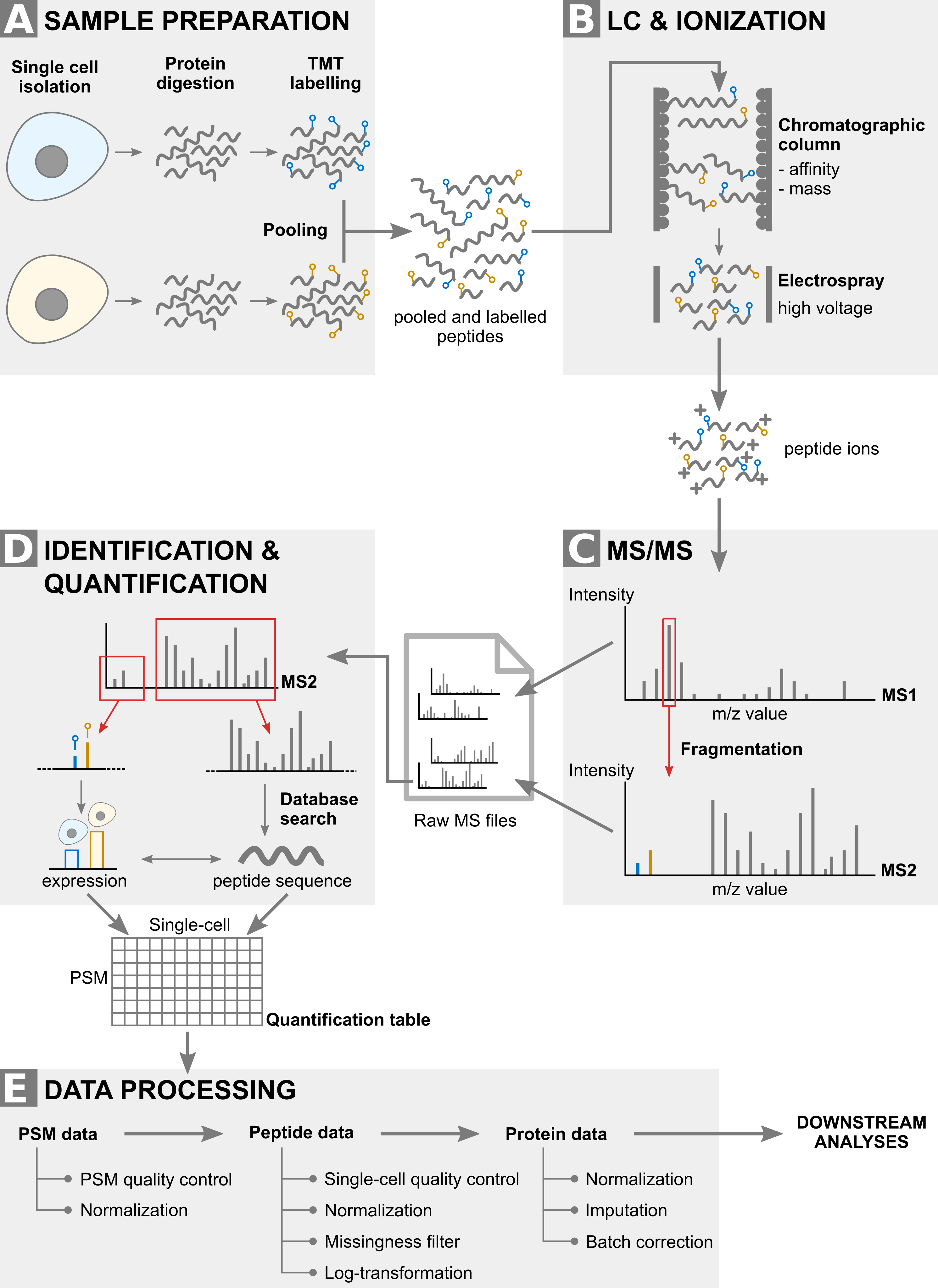
Main steps of the SCoPE2 data acquisition and processing pipeline.
The scp data framework
SCP data is very similar to bulk proteomics data with the exception that the PSM data may be composed of tens to hundreds of separate acquisition runs. The QFeatures class is able to store this acquisition structure by considering each MS run as a separate assay. Because the assays hold information about single cells, they are stored as SingleCellExperiment objects (Lun and Risso (2020)) to create a direct interface to existing Bioconductor packages. Performing downstream analyses (such as dimension reduction, clustering, finding markers) very easy. The links between related features across different assays are also stored to facilitate manipulation and visualization of of PSM, peptide and protein data as we go along with the processing workflow.
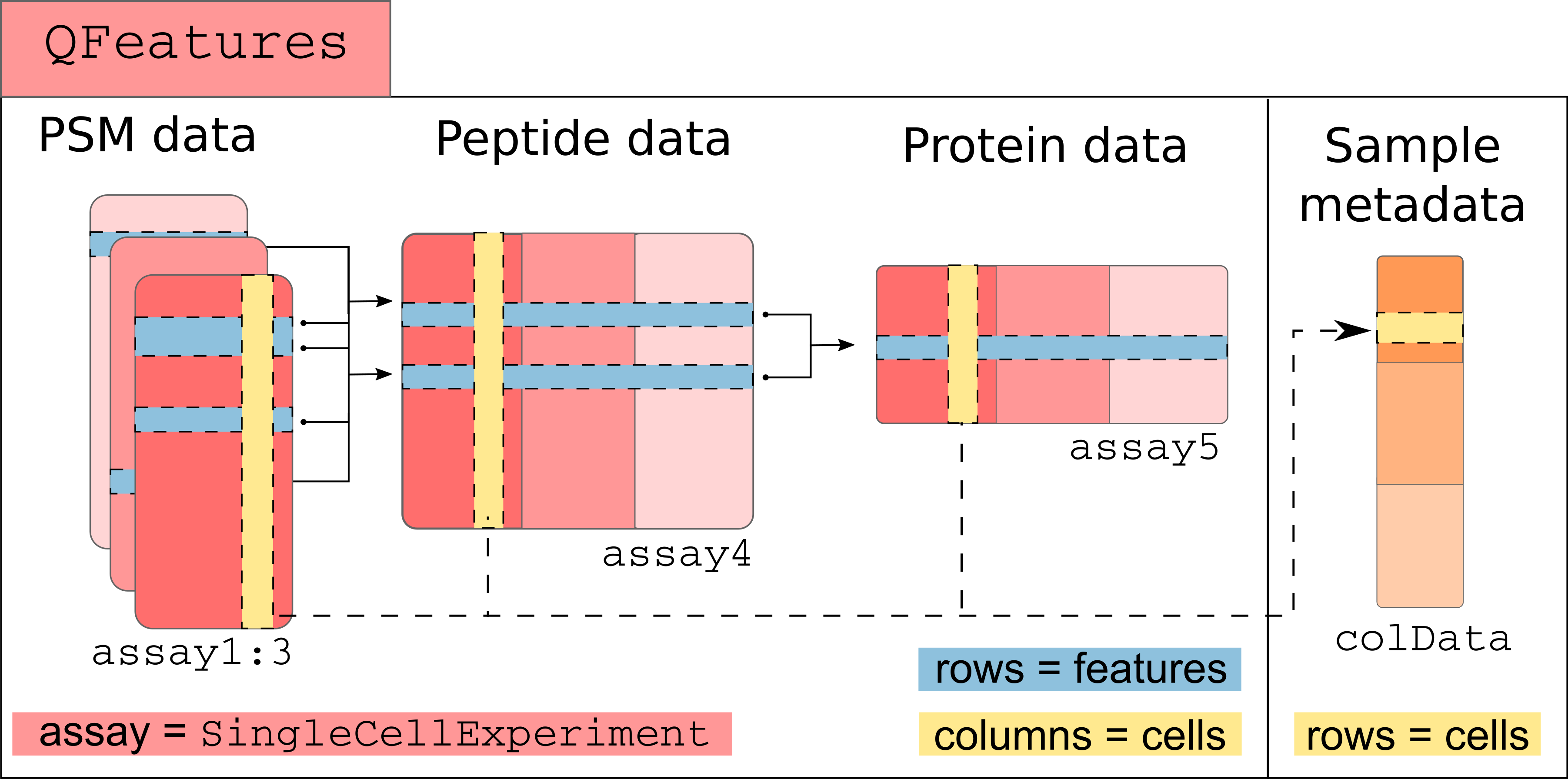
Conceptual overview of a QFeatures object containing SCP data. Each assay is stored as a SingleCellExperiment object.
The scp package
The general workflow for processing SCP data is very similar to the workflow for bulk proteomics that we presented in the previous vignette. Therefore, the QFeatures package already contains most of the tools required for the processing of SCP data. The scp package implements the missing functions that are specifically designed for dealing with SCP data. Below, we provide the list of functions from scp that extend the QFeatures functions:
-
readSCP: this is the main feature of thescppackage. It loads and formats standard data tables intoQFeaturesobjects ready for data processing. -
aggregateFeaturesOverAssays: extendsaggregateFeaturesto allow streamlined aggregation over multiple assays -
computeSCR: compute the sample over carrier ratio (SCR), a useful metric for feature QC -
divideByReference: divide columns by a reference column -
medianCVperCell: compute the median coefficient of variation (CV) per cell, a useful metric for single-cell QC -
normalizeSCP: extendsQFeatures::normalizetoSingleCellExperimentobjects -
pep2qvalue: compute q-values from posterior error probabilities -
rowDataToDF: extract therowDataof aQFeaturesobject to aDataFrame
We will demonstrate those functions later in this vignette.
Load SCP data
There are two input tables required for starting an analysis with scp: the feature data table and the sample annotation table.
Feature data
The feature data are generated after the identification and quantification of the MS spectra by a pre-processing software such as MaxQuant, ProteomeDiscoverer or MSFragger (the list of available software is actually much longer). We will here use as an example a data table that has been generated by MaxQuant. The table is available from the scp package and is called mqScpData (for MaxQuant-generated SCP data).
In this toy example, there are 1361 rows corresponding to features (quantified PSMs) and 149 columns corresponding to different data fields recorded by MaxQuant during the processing of the MS spectra.
Some of the columns contain quantitative data. In our example, those column names start with Reporter.intensity. followed by a number.
(quantCols <- grep("Reporter.intensity.\\d", colnames(mqScpData), value = TRUE))
##  [1] "Reporter.intensity.1"  "Reporter.intensity.2"  "Reporter.intensity.3"
##  [4] "Reporter.intensity.4"  "Reporter.intensity.5"  "Reporter.intensity.6"
##  [7] "Reporter.intensity.7"  "Reporter.intensity.8"  "Reporter.intensity.9"
## [10] "Reporter.intensity.10" "Reporter.intensity.11" "Reporter.intensity.12"
## [13] "Reporter.intensity.13" "Reporter.intensity.14" "Reporter.intensity.15"
## [16] "Reporter.intensity.16"
There are 16 columns with quantitative data because 16 labels were used during multiplexing. Let’s have a quick look into the quantitative data:
head(mqScpData[, quantCols])
##   Reporter.intensity.1 Reporter.intensity.2 Reporter.intensity.3
## 1                61251               501.71               3731.3
## 2                58648              1099.80               2837.7
## 3               150350              3705.00               9361.0
## 4                27347               405.90               1525.2
## 5                84035               583.09               4092.3
## 6                44895               700.23               2283.0
##   Reporter.intensity.4 Reporter.intensity.5 Reporter.intensity.6
## 1              1643.30               871.84               981.87
## 2               494.32               349.26              1030.50
## 3                 0.00              1945.40              1188.60
## 4                 0.00                 0.00               318.74
## 5               530.13               718.13              2204.50
## 6              1109.60                 0.00               675.79
##   Reporter.intensity.7 Reporter.intensity.8 Reporter.intensity.9
## 1              1200.10               939.06              1457.50
## 2                 0.00              1214.10               800.58
## 3              1574.00              2302.10              2176.10
## 4                 0.00               519.81                 0.00
## 5               960.51               453.77              1188.40
## 6                 0.00               809.38               668.88
##   Reporter.intensity.10 Reporter.intensity.11 Reporter.intensity.12
## 1               1329.80                981.83                    NA
## 2                807.79                391.38                    NA
## 3               1399.50               1307.50                2192.4
## 4                507.23                370.79                    NA
## 5                740.99                  0.00                    NA
## 6               1467.50                901.38                    NA
##   Reporter.intensity.13 Reporter.intensity.14 Reporter.intensity.15
## 1                    NA                    NA                    NA
## 2                    NA                    NA                    NA
## 3                1791.4                1727.5                2157.3
## 4                    NA                    NA                    NA
## 5                    NA                    NA                    NA
## 6                    NA                    NA                    NA
##   Reporter.intensity.16
## 1                    NA
## 2                    NA
## 3                  1398
## 4                    NA
## 5                    NA
## 6                    NA
Most columns in the mqScpData table contain feature metadata, that is data generated during the identification of the MS spectra. For instance, you may find the charge of the parent ion, the score and probability of a correct match between the MS spectrum and a peptide sequence, the sequence of the best matching peptide, its length, its modifications, the retention time of the peptide on the LC, the protein(s) the peptide originates from and much more.
head(mqScpData[, c("Charge", "Score", "PEP", "Sequence", "Length",
                   "Retention.time", "Proteins")])
##   Charge  Score        PEP    Sequence Length Retention.time
## 1      2 41.029 5.2636e-04   ATNFLAHEK      9         65.781
## 2      2 44.349 5.8789e-04   ATNFLAHEK      9         63.787
## 3      2 51.066 4.0315e-24 SHTILLVQPTK     11         71.884
## 4      2 63.816 4.7622e-06 SHTILLVQPTK     11         68.633
## 5      2 74.464 6.8709e-09 SHTILLVQPTK     11         71.946
## 6      2 41.502 5.3705e-02     SLVIPEK      7         76.204
##               Proteins
## 1 sp|P29692|EF1D_HUMAN
## 2 sp|P29692|EF1D_HUMAN
## 3  sp|P84090|ERH_HUMAN
## 4  sp|P84090|ERH_HUMAN
## 5  sp|P84090|ERH_HUMAN
## 6 sp|P62269|RS18_HUMAN
Finally, some columns may contain metadata related to the MS instrument. In MaxQuant, only the file names generated by the MS instrument are stored.
unique(mqScpData$Raw.file)
## [1] "190321S_LCA10_X_FP97AG"        "190222S_LCA9_X_FP94BM"
## [3] "190914S_LCB3_X_16plex_Set_21"  "190321S_LCA10_X_FP97_blank_01"
The 1361 PSM were found across 4 MS runs. While these 4 runs are contained in a single table, we prefer to split them in separate assay when building the QFeatures object, this will allow to have unique sample identifier that represent a combination of the MS run and the quantification column.
Sample annotation
Next to the feature, sample annotation contains the experimental design generated by the researcher. The rows of the sample annotation table correspond to a sample in the experiment and the columns correspond to the different pieces of available information. We will here use the second example table provided in scp:
data("sampleAnnotation")
head(sampleAnnotation)
##                Raw.file              Channel SampleType lcbatch sortday digest
## 1 190222S_LCA9_X_FP94BM Reporter.intensity.1    Carrier    LCA9      s8      N
## 2 190222S_LCA9_X_FP94BM Reporter.intensity.2  Reference    LCA9      s8      N
## 3 190222S_LCA9_X_FP94BM Reporter.intensity.3     Unused    LCA9      s8      N
## 4 190222S_LCA9_X_FP94BM Reporter.intensity.4   Monocyte    LCA9      s8      N
## 5 190222S_LCA9_X_FP94BM Reporter.intensity.5      Blank    LCA9      s8      N
## 6 190222S_LCA9_X_FP94BM Reporter.intensity.6   Monocyte    LCA9      s8      N
readSCP
readSCP is the function that converts the sample and the feature data into a QFeatures object following the data structure described above. The data belonging to each MS batch are stored in a separate SingleCellExperiment object, where feature metadata are stored in the rowData and the quantitative data are retrieved with assay(). The sample annotations are stored as the colData and are linked to the columns of each SingleCellExperiment object.
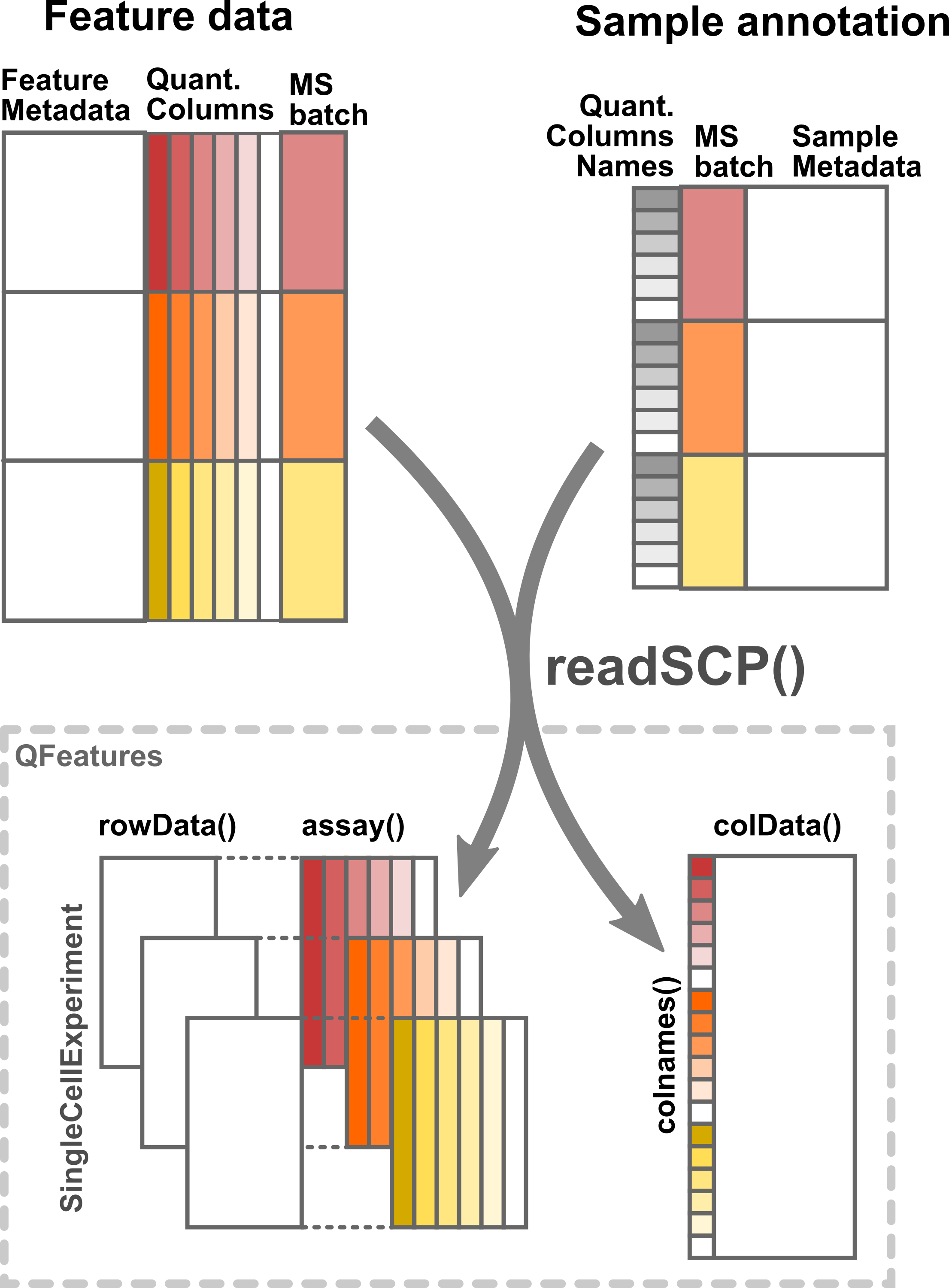
Illustration of the formatting by readSCP of the feature data table and the sample annotation table into a QFeatures object.
In practice, we provide the two tables to readSCP and tell the function which column holds the MS run information and which column in the sample annotation holds the quantitative column names in the feature data.
scp <- readSCP(featureData = mqScpData,
               colData = sampleAnnotation,
               batchCol = "Raw.file",
               channelCol = "Channel")
## Loading data as a 'SingleCellExperiment' object
## Splitting data based on 'Raw.file'
## Formatting sample metadata (colData)
## Formatting data as a 'QFeatures' object
scp
## An instance of class QFeatures containing 4 assays:
##  [1] 190222S_LCA9_X_FP94BM: SingleCellExperiment with 395 rows and 16 columns
##  [2] 190321S_LCA10_X_FP97_blank_01: SingleCellExperiment with 109 rows and 16 columns
##  [3] 190321S_LCA10_X_FP97AG: SingleCellExperiment with 487 rows and 16 columns
##  [4] 190914S_LCB3_X_16plex_Set_21: SingleCellExperiment with 370 rows and 16 columns
The object returned by readSCP is a QFeatures object containing 4 SingleCellExperiment assays that have been named after the 4 MS batches.
As mentioned in the previous vignette, sample data is retrieved from the colData. Note that unique sample names were automatically generated by combining the batch name and the column names of the quantitative data:
colData(scp)
## DataFrame with 64 rows and 6 columns
##                                                        Raw.file       Channel
##                                                     <character>   <character>
## 190222S_LCA9_X_FP94BMReporter.intensity.1         190222S_LC... Reporter.i...
## 190222S_LCA9_X_FP94BMReporter.intensity.2         190222S_LC... Reporter.i...
## 190222S_LCA9_X_FP94BMReporter.intensity.3         190222S_LC... Reporter.i...
## 190222S_LCA9_X_FP94BMReporter.intensity.4         190222S_LC... Reporter.i...
## 190222S_LCA9_X_FP94BMReporter.intensity.5         190222S_LC... Reporter.i...
## ...                                                         ...           ...
## 190914S_LCB3_X_16plex_Set_21Reporter.intensity.12 190914S_LC... Reporter.i...
## 190914S_LCB3_X_16plex_Set_21Reporter.intensity.13 190914S_LC... Reporter.i...
## 190914S_LCB3_X_16plex_Set_21Reporter.intensity.14 190914S_LC... Reporter.i...
## 190914S_LCB3_X_16plex_Set_21Reporter.intensity.15 190914S_LC... Reporter.i...
## 190914S_LCB3_X_16plex_Set_21Reporter.intensity.16 190914S_LC... Reporter.i...
##                                                    SampleType     lcbatch
##                                                   <character> <character>
## 190222S_LCA9_X_FP94BMReporter.intensity.1             Carrier        LCA9
## 190222S_LCA9_X_FP94BMReporter.intensity.2           Reference        LCA9
## 190222S_LCA9_X_FP94BMReporter.intensity.3              Unused        LCA9
## 190222S_LCA9_X_FP94BMReporter.intensity.4            Monocyte        LCA9
## 190222S_LCA9_X_FP94BMReporter.intensity.5               Blank        LCA9
## ...                                                       ...         ...
## 190914S_LCB3_X_16plex_Set_21Reporter.intensity.12  Macrophage        LCB3
## 190914S_LCB3_X_16plex_Set_21Reporter.intensity.13  Macrophage        LCB3
## 190914S_LCB3_X_16plex_Set_21Reporter.intensity.14  Macrophage        LCB3
## 190914S_LCB3_X_16plex_Set_21Reporter.intensity.15  Macrophage        LCB3
## 190914S_LCB3_X_16plex_Set_21Reporter.intensity.16  Macrophage        LCB3
##                                                       sortday      digest
##                                                   <character> <character>
## 190222S_LCA9_X_FP94BMReporter.intensity.1                  s8           N
## 190222S_LCA9_X_FP94BMReporter.intensity.2                  s8           N
## 190222S_LCA9_X_FP94BMReporter.intensity.3                  s8           N
## 190222S_LCA9_X_FP94BMReporter.intensity.4                  s8           N
## 190222S_LCA9_X_FP94BMReporter.intensity.5                  s8           N
## ...                                                       ...         ...
## 190914S_LCB3_X_16plex_Set_21Reporter.intensity.12          s9           R
## 190914S_LCB3_X_16plex_Set_21Reporter.intensity.13          s9           R
## 190914S_LCB3_X_16plex_Set_21Reporter.intensity.14          s9           R
## 190914S_LCB3_X_16plex_Set_21Reporter.intensity.15          s9           R
## 190914S_LCB3_X_16plex_Set_21Reporter.intensity.16          s9           R
The feature metadata is retrieved from the rowData. Since the feature metadata is specific to each assay, we need to tell from which assay we want to get the rowData:
rowData(scp[["190222S_LCA9_X_FP94BM"]])[, 1:5]
## DataFrame with 395 rows and 5 columns
##                   uid      Sequence    Length Modifications Modified.sequence
##           <character>   <character> <integer>   <character>       <character>
## PSM2    _(Acetyl (...     ATNFLAHEK         9 Acetyl (Pr...     _(Acetyl (...
## PSM4    _(Acetyl (... SHTILLVQPT...        11 Acetyl (Pr...     _(Acetyl (...
## PSM6    _(Acetyl (...       SLVIPEK         7 Acetyl (Pr...     _(Acetyl (...
## PSM9    _AAGLALK_ ...       AAGLALK         7    Unmodified         _AAGLALK_
## PSM12   _AALSAGK_ ...       AALSAGK         7    Unmodified         _AALSAGK_
## ...               ...           ...       ...           ...               ...
## PSM1242 _YSQVLANGL... YSQVLANGLD...        12    Unmodified     _YSQVLANGL...
## PSM1244 _YVLGPAVR_...      YVLGPAVR         8    Unmodified        _YVLGPAVR_
## PSM1247 _YYPTEDVPR...     YYPTEDVPR         9    Unmodified     _YYPTEDVPR...
## PSM1249 _YYSVNSR_ ...       YYSVNSR         7    Unmodified         _YYSVNSR_
## PSM1252 _YYTVFDR_ ...       YYTVFDR         7    Unmodified         _YYTVFDR_
Finally, we can also retrieve the quantification matrix for an assay of interest:
assay(scp, "190222S_LCA9_X_FP94BM")[1:5, 1:5]
##       190222S_LCA9_X_FP94BMReporter.intensity.1
## PSM2                                      58648
## PSM4                                      27347
## PSM6                                      44895
## PSM9                                     122070
## PSM12                                     58605
##       190222S_LCA9_X_FP94BMReporter.intensity.2
## PSM2                                    1099.80
## PSM4                                     405.90
## PSM6                                     700.23
## PSM9                                    1153.50
## PSM12                                    895.25
##       190222S_LCA9_X_FP94BMReporter.intensity.3
## PSM2                                     2837.7
## PSM4                                     1525.2
## PSM6                                     2283.0
## PSM9                                     7361.9
## PSM12                                    2763.8
##       190222S_LCA9_X_FP94BMReporter.intensity.4
## PSM2                                     494.32
## PSM4                                       0.00
## PSM6                                    1109.60
## PSM9                                    1732.30
## PSM12                                    867.82
##       190222S_LCA9_X_FP94BMReporter.intensity.5
## PSM2                                     349.26
## PSM4                                       0.00
## PSM6                                       0.00
## PSM9                                    1515.60
## PSM12                                   1050.30
The scpdata package
Next to scp, we also developed scpdata, a data package that disseminates published SCP data sets formatted using the scp data structure. The package heavily relies on the ExperimentHub infrastructure. This package is an ideal platform for data sharing and promotes for open and reproducible science in SCP, it facilitates the access for developers to SCP data to build and benchmark new methodologies and it facilitates the access for new users to data in the context of training and demonstration (like this workshop).
After loading the package, you can have a look at the available datasets by running:
library(scpdata)
scpdata()
## DataFrame with 12 rows and 15 columns
##                title  dataprovider       species taxonomyid      genome
##          <character>   <character>   <character>  <integer> <character>
## EH3899 specht2019... SlavovLab ... Homo sapie...       9606          NA
## EH3900 specht2019... SlavovLab ... Homo sapie...       9606          NA
## EH3901 dou2019_ly...       MassIVE Homo sapie...       9606          NA
## EH3902 dou2019_mo...       MassIVE Mus muscul...      10090          NA
## EH3903 dou2019_bo...       MassIVE Mus muscul...      10090          NA
## ...              ...           ...           ...        ...         ...
## EH3906 zhu2018NC_...         PRIDE Homo sapie...       9606          NA
## EH3907 zhu2018NC_...         PRIDE Homo sapie...       9606          NA
## EH3908    cong2020AC         PRIDE Homo sapie...       9606          NA
## EH3909     zhu2019EL         PRIDE Gallus gal...       9031          NA
## EH6011 liang2020_...         PRIDE Homo sapie...       9606          NA
##          description coordinate_1_based    maintainer rdatadateadded
##          <character>          <integer>   <character>    <character>
## EH3899 SCP expres...                  1 Christophe...     2020-11-05
## EH3900 SCP expres...                  1 Christophe...     2020-11-05
## EH3901 SCP expres...                  1 Christophe...     2020-11-05
## EH3902 SCP expres...                  1 Christophe...     2020-11-05
## EH3903 SCP expres...                  1 Christophe...     2020-11-05
## ...              ...                ...           ...            ...
## EH3906 Near SCP e...                  1 Christophe...     2020-11-05
## EH3907 Near SCP e...                  1 Christophe...     2020-11-05
## EH3908 SCP expres...                  1 Christophe...     2020-11-05
## EH3909 SCP expres...                  1 Christophe...     2020-11-05
## EH6011 Expression...                  1 Christophe...     2021-04-27
##        preparerclass                                          tags  rdataclass
##          <character>                                        <list> <character>
## EH3899       scpdata Experiment...,Expression...,Experiment...,...   QFeatures
## EH3900       scpdata Experiment...,Expression...,Experiment...,...   QFeatures
## EH3901       scpdata Experiment...,Expression...,Experiment...,...   QFeatures
## EH3902       scpdata Experiment...,Expression...,Experiment...,...   QFeatures
## EH3903       scpdata Experiment...,Expression...,Experiment...,...   QFeatures
## ...              ...                                           ...         ...
## EH3906       scpdata Experiment...,Expression...,Experiment...,...   QFeatures
## EH3907       scpdata Experiment...,Expression...,Experiment...,...   QFeatures
## EH3908       scpdata Experiment...,Expression...,Experiment...,...   QFeatures
## EH3909       scpdata Experiment...,Expression...,Experiment...,...   QFeatures
## EH6011       scpdata      Expression...,MassSpectr...,Proteome,...   QFeatures
##            rdatapath     sourceurl  sourcetype
##          <character>   <character> <character>
## EH3899 scpdata/sp... https://sc...         CSV
## EH3900 scpdata/sp... https://sc...         CSV
## EH3901 scpdata/do... ftp://mass...    XLS/XLSX
## EH3902 scpdata/do... ftp://mass...    XLS/XLSX
## EH3903 scpdata/do... ftp://mass...    XLS/XLSX
## ...              ...           ...         ...
## EH3906 scpdata/zh... ftp://ftp....         TXT
## EH3907 scpdata/zh... ftp://ftp....         TXT
## EH3908 scpdata/co... ftp://ftp....         TXT
## EH3909 scpdata/zh... ftp://ftp....         TXT
## EH6011 scpdata/li... ftp://ftp....         TXT
For instance, loading the data sets published in Zhu et al. (2019) is as simple as calling the title of the data set:
zhu2019EL()
## An instance of class QFeatures containing 62 assays:
##  [1] 1H1a: SingleCellExperiment with 152 rows and 1 columns
##  [2] 1H1b: SingleCellExperiment with 267 rows and 1 columns
##  [3] 1H1c: SingleCellExperiment with 128 rows and 1 columns
##  ...
##  [60] 2N0c: SingleCellExperiment with 61 rows and 1 columns
##  [61] peptides: SingleCellExperiment with 3444 rows and 60 columns
##  [62] proteins: SingleCellExperiment with 840 rows and 60 columns
Reproduce a published analysis
As a use-case, we will reproduce the analysis of the SCoPE2 data published in Specht et al. (2021). SCoPE2 is the first published SCP protocol that has been used to profile thousands of proteins in thousands of single-cells. This is a technical milestone for the field and it opens the door for a fine-grain understanding of biological processes at the protein level.
Along their acquisition protocol, the authors have also provided an R script to reproduce their data processing. The code is hard to read and built from scratch. We have used scp to standardize this workflow (Vanderaa and Gatto (2021)) and reproduce the results using code that can easily be adapted to other data sets. The outline of the workflow is shown below.
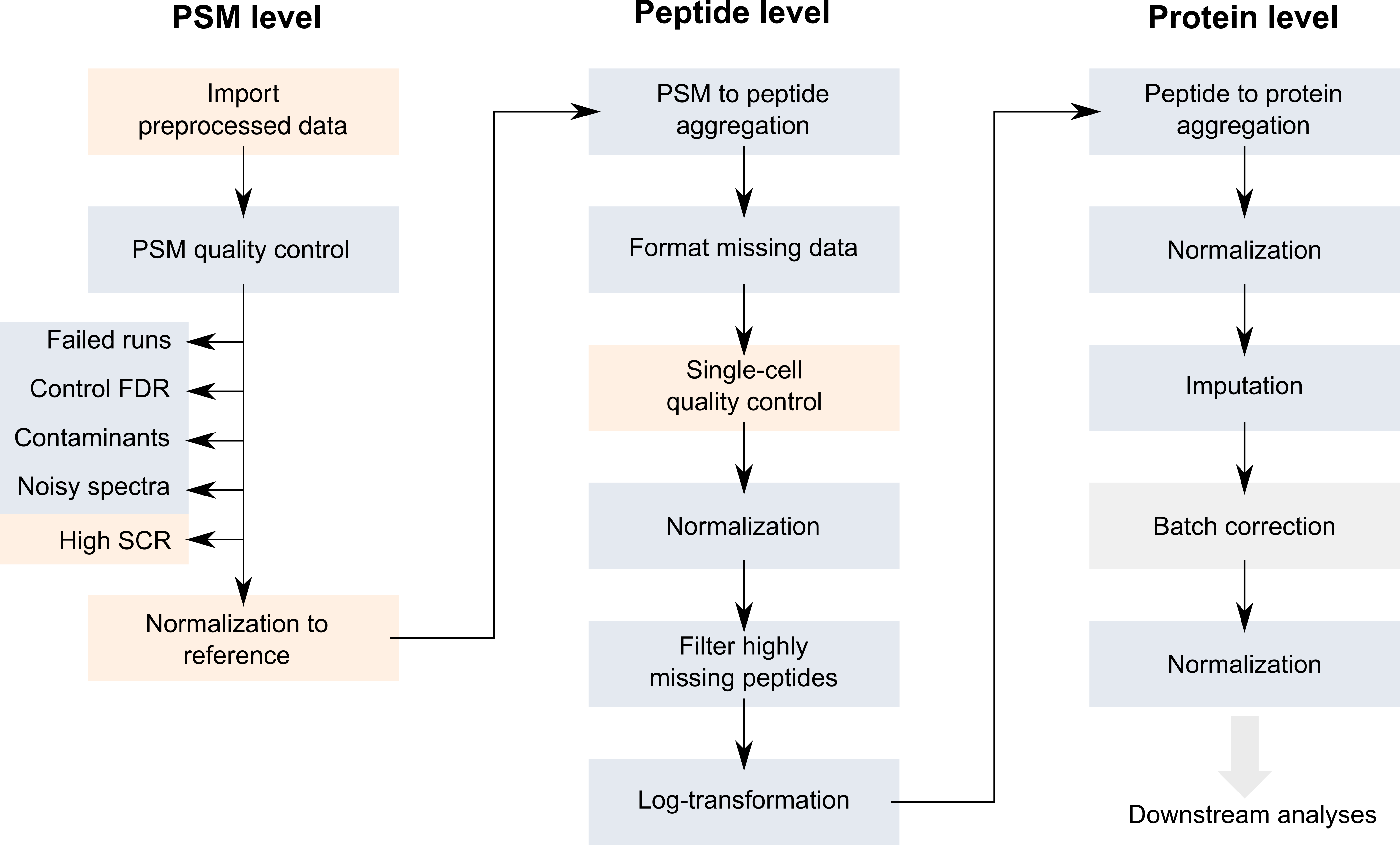
Workflow describing the main steps performed by Specht et al. to process the SCP data. Figure taken from Vanderaa and Gatto (2021)
The replication analysis on the full data set is provided in another vignette.
Before we start
The remainder of the vignette includes a few exercises for you to have your hands on the functions in QFeatures and scp. We have hidden the solution under Solution ticks that you can click on to reveal a good answer (sometimes, several solution are possible but we provided only one). You can also make use of some hints and fill-the-blank if you feel you are getting stuck. Each exercise has an associated data that you can load upfront. This will avoid you to rerun the whole vignette for every exercise.
Also, to reduce the computational burden, we will focus the replication only on a part of the SCoPE2 data. You can find the full replication in another vignette (Vanderaa and Gatto (2021))
Import the data
In a previous section we have shown how to format the feature and sample tables to a Qfeatures object for a small subset of the SCoPE2 data set. We will here import the data directly from scpdata to gain some time.
(scope2 <- specht2019v3())
## An instance of class QFeatures containing 179 assays:
##  [1] 190222S_LCA9_X_FP94AA: SingleCellExperiment with 2777 rows and 11 columns
##  [2] 190222S_LCA9_X_FP94AB: SingleCellExperiment with 4348 rows and 11 columns
##  [3] 190222S_LCA9_X_FP94AC: SingleCellExperiment with 4917 rows and 11 columns
##  ...
##  [177] 191110S_LCB7_X_APNOV16plex2_Set_9: SingleCellExperiment with 4934 rows and 16 columns
##  [178] peptides: SingleCellExperiment with 9354 rows and 1490 columns
##  [179] proteins: SingleCellExperiment with 3042 rows and 1490 columns
The data set provides 177 assays containing the PSM data, but also two assays that contain the peptide and protein data generated by the authors in the original work. We will here work only on samples acquired as part of the LCB3 batch.
PSM quality control
This section will guide you through the filtering of low-quality features based on different metrics.
Filter out failed runs based on PSM content
First, only the assays that have sufficient PSMs are kept. The authors keep an assay if it has over 500 PSMs. Before filtering, let’s first look at the distribution of the number of PSMs per assay. You can extract the number of rows (here PSMs) and the number of columns (TMT channels) of each assay using the dims function implemented in QFeatures.
nPSMs <- dims(lcb3)[1, ]Let’s have a look at the number of features that were identified in the different runs. The data visualization in this vignette is performed using the ggplot2 function.
library("ggplot2")
ggplot(data.frame(nPSMs)) +
    aes(x = nPSMs) +
    geom_histogram() +
    geom_vline(xintercept = 500)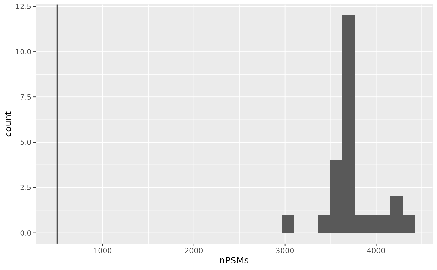
No MS run failed in the LB3 batch. If some runs had failed, we could have subset the data taking advantage of the subsetting method of a QFeatures object.
lcb3 <- lcb3[, , nPSMs > 500]Filter out contaminants
All MS-based proteomic experiment is subjected to contamination from the environment. The most common contamination is keratin released from the researcher’s skin. A small database of known contaminants is commonly supplied to tag PSMs originating from potential contaminants. Next to that, a decoy database consisting of reversed peptide sequence is used to assess the reliability of the PSM identification and tag false hits.
You can remove the PSMs that were matched to contaminant proteins (the protein name starts with CON) or to the decoy database (the protein name starts with REV) using the filterFeatures function (cf previous vignette). To match the protein identifiers, you can use the grepl function and the filterFeatures will automatically retrieve the requested variable from the rowData.
lcb3 <- filterFeatures(lcb3,
                       ~ !grepl("REV|CON", protein))
Filter out PSMs with high false discovery rate
Next, the SCoPE2 workflow filters PSMs based on the false discovery rate (FDR) for identification. This will remove the PSMs that were matched by chance. The PSM data were already processed with DART-ID (Chen, Franks, and Slavov (2019)), a python software that updates the confidence in peptide identification using an Bayesian inference approach. DART-ID outputs for every PSM the updated posterior error probability (PEP). Filtering on the PEP is too conservative and it is rather advised to filter based on FDR (Käll et al. (2008)). To control for the FDR, we need to compute q-values, that correspond to the minimal FDR threshold that would still select the associated feature.
The scp package provides some utility function to compute common metrics and statistics from the rowData that are automatically added to the rowData. Converting PEPs to q-values is one such example. You can use the pep2qvalue function to easily convert PEPs to q-values. We here compute the q-values from the dart_PEP and store the result in the rowData of each assay under qvalue_psm.
lcb3 <- pep2qvalue(lcb3,
                   i = names(lcb3),
                   PEP = "dart_PEP",
                   rowDataName = "qvalue_psm")
You can also compute de protein-level q-values when providing the protein name (taken from the rowData) as a grouping variable.
lcb3 <- pep2qvalue(lcb3,
                   i = names(lcb3),
                   groupBy = "protein",
                   PEP = "dart_PEP",
                   rowDataName = "qvalue_protein")
Now that we have q-values available in the rowData, we can use them to filter out low-confidence PSMs using filterFeatures. The SCoPE2 authors removed features so to control a 1% PSM and protein FDR.
lcb3 <- filterFeatures(lcb3,
                       ~ qvalue_psm < 0.01 & qvalue_protein < 0.01)
Filter out PSMs with high sample to carrier ratio
The SCoPE2 authors suggested in their paper a new PSM quality control for SCP data: the sample to carrier ratio (SCR). The SCR is computed for every PSM separately as the (mean) intensity of the single-cell samples divided by the intensity of the carrier (200 cells) acquired during the same run as the sample. It is expected that the carrier intensities are much higher than the single-cell intensities.
computeSCR is another example of utility function from the scp package. It can be used to automatically compute the SCR for each PSM in the assays of interest. All that is required is to provide the function a way to tell what sample is what. You can achieve this thanks to the sample annotations contained in the colData. In this dataset, SampleType gives the type of sample that is present in each TMT channel. The SCoPE2 protocol includes 5 types of samples:
table(lcb3$SampleType)
##
##      Blank    Carrier Macrophage   Monocyte  Reference     Unused
## 22 24 192 74 24 48- The carrier channels (
Carrier) contain 200-cell equivalents and are meant to boost the peptide identification rate. - The normalization channels (
Reference) contain 5 cell equivalents and are used to partially correct for between-run variation. - The unused channels (
Unused) are channels that are left empty due to isotopic cross-contamination by the carrier channel. - The blank channels (
Blank) contain samples that do not contain any cell but are processed as single-cell samples. - The single-cell sample channels contain the single-cell samples of interest (
MacrophageorMonocyte).
The computeSCR function expects the user to provide a pattern (following regular expression syntax) that identifies the carrier column(s) (carrierPattern) a pattern that identifies the sample columns (samplePattern). The function will store the computed SCRs of each PSM in the rowData of the corresponding assay. When multiple matches are found for samples or carrier, you can also provide a summarizing function through sampleFUN and carrierFUN, respectively.
Exercise: It’s your turn now, compute the SCR by considering blanks, monocytes and macrophages as samples of interest. Note there are multiple samples per run for each PSM and you should therefore compute the mean of the samples. There is only a single carrier, so you don’t need to bother providing carrierFUN.
data("lcb3_1")
lcb3 <- lcb3_1
Hint 1
Remember that the sample types are available from thecolData column SampleType. The output above provides an overview of the available sample types in the data.
Hint 2
Mutliple samples of interest should match your pattern in each per assay. You can provide a function or a string referring to a function tosampleFUN.
Fill the blank 1
lcb3 <- computeSCR(lcb3,
                   i = names(lcb3),
                   colvar = ...,
                   carrierPattern = ...,
                   samplePattern = ...,
                   sampleFUN = ...,
                   rowDataName = "MeanSCR")
Fill the blank 2
lcb3 <- computeSCR(lcb3,
                   i = names(lcb3),
                   colvar = ...,
                   carrierPattern = "Carrier",
                   samplePattern = "Blank|Monocyte|Macrophage",
                   sampleFUN = ...,
                   rowDataName = "MeanSCR")
Solution
lcb3 <- computeSCR(lcb3,
                   i = names(lcb3),
                   colvar = "SampleType",
                   carrierPattern = "Carrier",
                   samplePattern = "Blank|Monocyte|Macrophage",
                   sampleFUN = mean,
                   rowDataName = "MeanSCR")
Before applying the filter, let’s plot the distribution of the mean SCR. You can extract the MeanSCR from the rowData of several assays using the rbindRowData function. It takes the rowData of interest and returns a single DataFrame table with all rowData variables common to the selected assays.
rbindRowData(lcb3, i = names(lcb3)) %>%
    data.frame %>%
    ggplot(aes(x = MeanSCR)) +
    geom_histogram() +
    geom_vline(xintercept = c(1/200, 0.1),
               lty = 2:1) +
    scale_x_log10()
## Warning: Transformation introduced infinite values in continuous x-axis
## Warning: Removed 2832 rows containing non-finite values (stat_bin).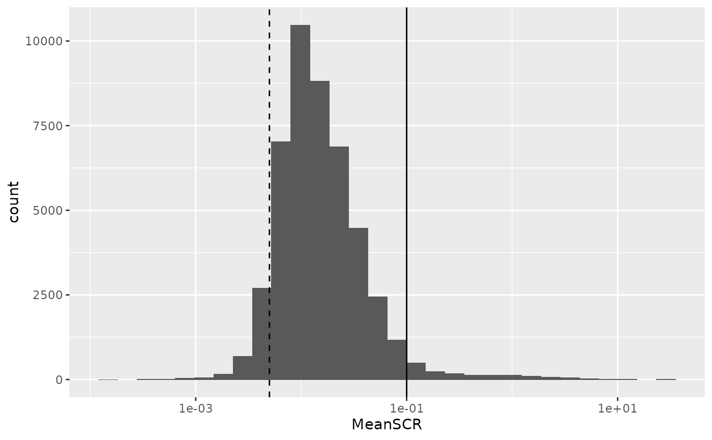
A great majority of the PSMs have a mean SCR that is lower than 10%, as expected. The mode of the distribution is located close to 1%, as expected since every carrier sample contains 200 cells leading to an expected ratio of 0.5% (dashed line).
Exercise: keep only PSMs that have a mean SCR lower than 10%. Make sure also to remove mean SCR values that are NA (due to missing quantification data or to dividing zero by zero) or infinite (when carrier is zero but not samples).
Hint 1
We already used thefilterFeatures function a few times in this vignette, take inspiration from the previous sections.
Hint 2
You can check whether the mean SCR is NA usingis.na(MeanSCR), and similarly is.infinite(MeanSCR) for infinite values.
Fill the blank
lcb3 <- filterFeatures(lcb3,
                       ~ !is.na(MeanSCR) &
                           !is.infinite(MeanSCR) &
                           ...)
Solution
lcb3 <- filterFeatures(lcb3,
                       ~ !is.na(MeanSCR) &
                           !is.infinite(MeanSCR) &
                           MeanSCR < 0.1)
Filter out PSMs with noisy spectra
A PIF (parental ion fraction) smaller than 80 % indicates the associated spectra is contaminated by co-isolated peptides and therefore the quantification becomes unreliable. The PIF was computed by MaxQuant and is readily available for filtering. Using again filterFeatures, we keep only PSMs that have low spectral contamination, that is, PSMs with an associated PIF greater than 0.8.
lcb3 <- filterFeatures(lcb3,
                       ~ !is.na(PIF) & PIF > 0.8)
Normalization to reference
In order to partially correct for between-run variation, the SCoPE2 authors compute relative reporter ion intensities. This means that intensities measured for single-cells are divided by the reference channel (5-cell equivalents). Before normalization:
assay(lcb3[[1]])[1:5, 1:5]
##         190913S_LCB3_X_16plex_Set_12_RI1 190913S_LCB3_X_16plex_Set_12_RI2
## PSM149                            112830                           3638.1
## PSM1114                           352770                          10268.0
## PSM2144                           179260                           4943.6
## PSM2703                           247810                           6965.6
## PSM3259                           240900                           8922.6
##         190913S_LCB3_X_16plex_Set_12_RI3 190913S_LCB3_X_16plex_Set_12_RI4
## PSM149                            5805.9                             0.00
## PSM1114                          19621.0                             0.00
## PSM2144                           8769.5                             0.00
## PSM2703                          10308.0                             0.00
## PSM3259                          16451.0                           360.84
##         190913S_LCB3_X_16plex_Set_12_RI5
## PSM149                            1012.9
## PSM1114                           1974.0
## PSM2144                           1193.9
## PSM2703                           1094.8
## PSM3259                           3423.6
You can use the divideByReference function that divides channels of interest by the reference channel. Similarly to computeSCR, you can point to the samples and the reference columns in each assay using the annotation contained in the colData.
lcb3 <- divideByReference(lcb3,
                          i = names(lcb3),
                          colvar = "SampleType",
                          samplePattern = ".",
                          refPattern = "Reference")
After normalization:
assay(lcb3[[1]])[1:5, 1:5]
##         190913S_LCB3_X_16plex_Set_12_RI1 190913S_LCB3_X_16plex_Set_12_RI2
## PSM149                          31.01344                                1
## PSM1114                         34.35625                                1
## PSM2144                         36.26102                                1
## PSM2703                         35.57626                                1
## PSM3259                         26.99886                                1
##         190913S_LCB3_X_16plex_Set_12_RI3 190913S_LCB3_X_16plex_Set_12_RI4
## PSM149                          1.595860                       0.00000000
## PSM1114                         1.910888                       0.00000000
## PSM2144                         1.773910                       0.00000000
## PSM2703                         1.479844                       0.00000000
## PSM3259                         1.843745                       0.04044113
##         190913S_LCB3_X_16plex_Set_12_RI5
## PSM149                         0.2784146
## PSM1114                        0.1922478
## PSM2144                        0.2415042
## PSM2703                        0.1571724
## PSM3259                        0.3836998
PSM to peptide aggregation
Now that the PSM assays are processed, you can aggregate them to peptides. This is performed using the aggregateFeaturesOverAssays function. This is a wrapper function in scp that sequentially calls the aggregateFeatures from the QFeatures package over the different assays. For each assay, the function aggregates several PSMs into a unique peptide given an aggregating variable in the rowData (peptide sequence) and a user-supplied aggregating function (the median for instance). Regarding the aggregating function, the SCoPE2 analysis removes duplicated peptide sequences per run by taking the first non-missing value. While better alternatives are documented in QFeatures::aggregateFeatures, we suggest to use this approach for the sake of replication, but also to illustrate that custom functions can be applied when aggregating.
For each assay, a new aggregated assay will be added to the dataset. The aggregated peptide assays must be given a name. We here suggest to use the original names prefixed with peptides_.
You now have all the required information to aggregate the PSMs to peptides.
Exercise: use the aggregateFeaturesOverAssays function to aggregate PSMs to peptides. Don’t forget to provide the remove.duplicates as an aggregating function.
data("lcb3_2")
lcb3 <- lcb3_2
Hint
You should aggregate PSMs to peptides. So, you can group the PSMs by supplyingfcol = "peptide". The function will take the peptide column in the rowData that contains the peptide sequences and create a new aggregated feature for each unique sequence.
Fill the blank
lcb3 <- aggregateFeaturesOverAssays(lcb3,
                                    i = names(lcb3),
                                    fcol = "peptide",
                                    name = ...,
                                    fun = ...)
Solution
lcb3 <- aggregateFeaturesOverAssays(lcb3,
                                    i = names(lcb3),
                                    fcol = "peptide",
                                    name = peptideAssays,
                                    fun = remove.duplicates)
lcb3
## An instance of class QFeatures containing 48 assays:
##  [1] 190913S_LCB3_X_16plex_Set_12: SingleCellExperiment with 1621 rows and 16 columns
##  [2] 190913S_LCB3_X_16plex_Set_17_reinject2: SingleCellExperiment with 1484 rows and 16 columns
##  [3] 190914S_LCB3_X_16plex_Set_1: SingleCellExperiment with 1415 rows and 16 columns
##  ...
##  [46] peptides_190914S_LCB3_X_16plex_Set_7: SingleCellExperiment with 1771 rows and 16 columns
##  [47] peptides_190914S_LCB3_X_16plex_Set_8: SingleCellExperiment with 1348 rows and 16 columns
##  [48] peptides_190914S_LCB3_X_16plex_Set_9: SingleCellExperiment with 1944 rows and 16 columns
There are as many new assay that are added as there are assays to aggregate. Under the hood, the QFeatures architecture preserves the relationship between the aggregated assays. See ?AssayLinks for more information on relationships between assays.
It is now time to have an overview of our data set:
plot(lcb3)
Exercise: there are too many assays displayed on the graph above that is becoming too crowded. The plot function also provides an interactive version of this graph that you can explore manually. Search the documentation and create an interactive plot for the lcb3 data.
Solution
plot(lcb3, interactive = TRUE)Cleaning missing data
The next step is to replace zero and infinite values by NAs. The zeros can be biological zeros or technical zeros and differentiating between the two types is a difficult task, they are therefore better considered as missing data that should be modelled using dedicated methods. The infinite values appear during the normalization by the reference when the reference channel is zero. This artefact could easily be avoided if we had replaced the zeros by NAs at the beginning of the workflow, what we strongly recommend for future analyses.
The infIsNA and the zeroIsNA functions automatically detect infinite and zero values, respectively, and replace them with NAs. Those two functions are provided by the QFeatures package. See here how you can replace infinite values by NA:
sum(is.infinite(assay(lcb3, peptideAssays[1])))
## [1] 31
lcb3 <- infIsNA(lcb3, i = peptideAssays)
sum(is.infinite(assay(lcb3, peptideAssays[1])))
## [1] 0
You can also replace all zero values by NA.
Join the peptide assays in one assay
Up to now, the data belonging to each MS run are kept in separate assays. You can combine all batches into a single assay using the joinAssays function from the QFeatures package.
lcb3 <- joinAssays(lcb3,
                   i = peptideAssays,
                   name = "peptides")
Note joinAssays has created a new assay called peptides that combines the previously aggregated peptide assays.
lcb3
## An instance of class QFeatures containing 49 assays:
##  [1] 190913S_LCB3_X_16plex_Set_12: SingleCellExperiment with 1621 rows and 16 columns
##  [2] 190913S_LCB3_X_16plex_Set_17_reinject2: SingleCellExperiment with 1484 rows and 16 columns
##  [3] 190914S_LCB3_X_16plex_Set_1: SingleCellExperiment with 1415 rows and 16 columns
##  ...
##  [47] peptides_190914S_LCB3_X_16plex_Set_8: SingleCellExperiment with 1348 rows and 16 columns
##  [48] peptides_190914S_LCB3_X_16plex_Set_9: SingleCellExperiment with 1944 rows and 16 columns
##  [49] peptides: SingleCellExperiment with 4365 rows and 384 columns
At this point, you can regularly have a look at plot(lcb3, interactive = TRUE) to keep an overview of the assay hierarchy.
Single-cell quality control
The SCoPE2 workflow proceeds with the filtering of low quality cells. The filtering is based on the median coefficient of variation (CV) per cell. The CV is measured for each protein in each sample as the standard deviation of the peptide quantifications belonging to the same protein divided by the average expression of those peptides. Taking the median CV per cell will give a measure of the robustness of the quantification within that cell. We want to remove cells that exhibit a high median CV because inconsistent measures imply artefacts during samples preparation.
This is performed using the medianCVperCell function from the scp package. The function takes the protein information from the rowData of the assays. This information will tell how to group the features (peptides) when computing the CV. The SCoPE2 authors applied a custom normalization (norm = "SCoPE2") to the data prior to computing CVs and they computed CVs only if at least 6 peptides are available (nobs = 6). See the methods section in Specht et al. (2021) for more information.
lcb3 <- medianCVperCell(lcb3,
                        i = peptideAssays,
                        groupBy = "protein",
                        nobs = 6,
                        colDataName = "MedianCV",
                        norm = "SCoPE2")
The computed CVs are stored in the colData. We can now filter cells that have reliable quantifications. The blank samples are not expected to have reliable quantifications and hence can be used to estimate a null distribution of the CV. This distribution helps defining a threshold that filters out single-cells that contain noisy quantification.
colData(lcb3) %>%
    data.frame %>%
    filter(SampleType %in% c("Macrophage",  "Monocyte", "Blank")) %>%
    ggplot(aes(x = MedianCV,
               fill = SampleType)) +
    geom_histogram() +
    geom_vline(xintercept = 0.365)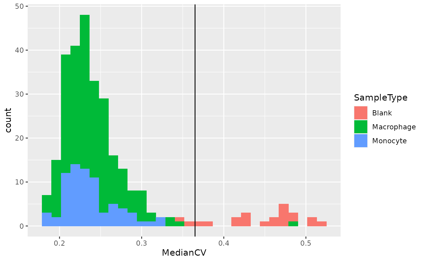
We can see that the protein quantification for single-cells are much more consistent within single-cell channels than within blank channels. A threshold of 0.365 best separates single-cells from empty channels.
Exercise: keep cells that have a median CV lower than 0.365. You should also keep macrophages and monocytes as those represent the samples of interest. You can easily achieve this by subsetting the samples based on the associated colData using the subsetByColData function from the MultiAssayExperiment package.
data("lcb3_3")
lcb3 <- lcb3_3
Fill the blanks
lcb3 <- subsetByColData(lcb3,
                        lcb3$MedianCV ... &
                            lcb3$SampleType ...)
Solution
lcb3 <- subsetByColData(lcb3,
                        lcb3$MedianCV < 0.365 &
                            lcb3$SampleType %in% c("Macrophage", "Monocyte"))
Normalization
Although you already normalized by the reference channels, the authors of SCoPE2 suggested to proceed with further data normalization. First, they normalize the columns (samples) of the peptide data by the median intensities. Then, the rows (peptides) are normalized by dividing the relative intensities by the mean relative intensities.
## Scale column with median
lcb3 <- normalizeSCP(lcb3,
                     i = "peptides",
                     method = "div.median",
                     name = "peptides_norm1")
The second normalization method is not available in normalize, but you can still apply it using the sweep method from the QFeatures package that is inspired from the base::sweep function. We here show how to use it, note that is it a bit more complicated since you need to manually provide the scaling factors.
sf <- rowMeans(assay(lcb3[["peptides_norm1"]]), na.rm = TRUE)
## Scale rows with mean
lcb3 <- sweep(lcb3,
              i = "peptides_norm1", MARGIN = 1,
              FUN = "/",
              STATS = sf,
              name = "peptides_norm2")
Each normalization step is stored in a separate assay. You can have a look at the QFeatures plot as suggested previously.
Filter highly missing peptides
Peptides that contain many missing values are not informative. Therefore, it is advised to remove highly missing peptides from downstream analysis. The SCoPE2 authors removed peptides with more than 99 % missing data. You can achieve this using the filterNA function from QFeatures.
lcb3 <- filterNA(lcb3,
                 i = "peptides_norm2",
                 pNA = 0.99)
Log-transformation
The last processing step of the peptide data before aggregating to proteins is to log2-transform the data.
lcb3 <- logTransform(lcb3,
                     base = 2,
                     i = "peptides_norm2",
                     name = "peptides_log")
Peptide to protein aggregation
Similarly to aggregating PSM data to peptide data, you can aggregate peptide data to protein data. Note this time, you can use the aggregateFeatures function instead of the aggregateFeaturesOverAssays function since you only need to aggregate only one assay (peptides_log).
lcb3 <- aggregateFeatures(lcb3,
                          i = "peptides_log",
                          name = "proteins",
                          fcol = "protein",
                          fun = matrixStats::colMedians, na.rm = TRUE)
Normalization
Normalization is performed similarly to peptide normalization. You can use the same functions, but since the data were log-transformed at the peptide level, you should subtract/center by the statistic (median or mean) instead of dividing.
## Center columns with median
lcb3 <- normalizeSCP(lcb3,
                     i = "proteins",
                     method = "center.median",
                     name = "proteins_norm1")
## Center rows with mean
lcb3 <- sweep(lcb3,
              i = "proteins_norm1",
              MARGIN = 1,
              FUN = "-",
              STATS = rowMeans(assay(lcb3[["proteins_norm1"]]),
                               na.rm = TRUE),
              name = "proteins_norm2")
Imputation
The protein data contains a lot of missing values. Let’s have a look at the distribution of the percent missing data per sample. You can easily achieve this by using the nNA function. Cells contain on average between 60 and 70% missing values!
nNAres <- nNA(lcb3, "proteins_norm2")$nNAcols
ggplot(data.frame(nNAres),
       aes(x = pNA)) +
    geom_histogram()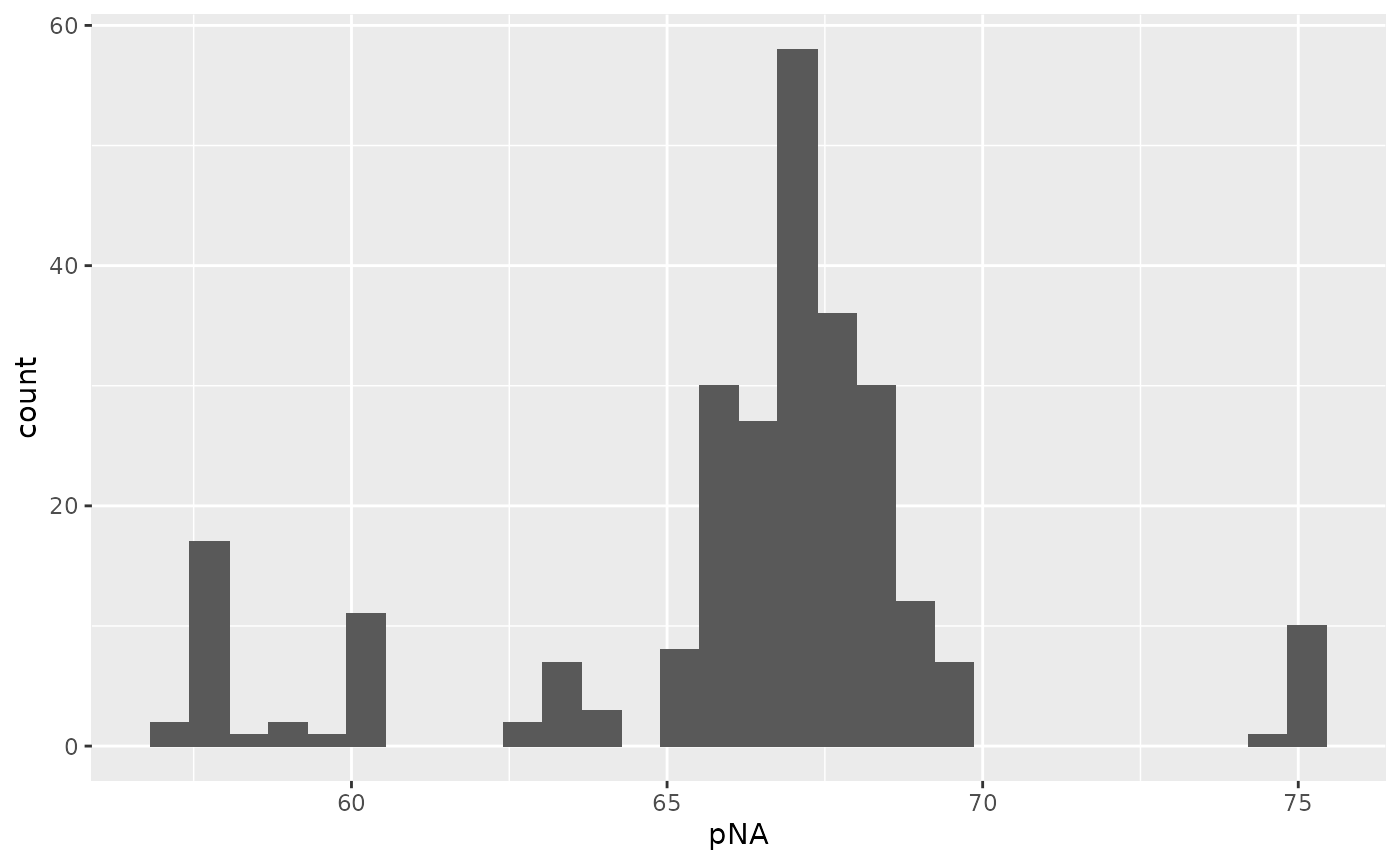
The missing data is imputed using K nearest neighbors. QFeatures provides the impute function that serves as an interface to different imputation algorithms among which the KNN algorithm from impute::impute.knn.
lcb3 <- impute(lcb3,
               i = "proteins_norm2",
               method = "knn",
               k = 3, rowmax = 1, colmax= 1,
               maxp = Inf, rng.seed = 1234)
Batch correction
The final step is to model the remaining batch effects and correct for it. The data were acquired as a series of MS runs. Each MS run can be subjected to technical perturbations that lead to differences in the data. This must be accounted for to avoid attributing biological effects to technical effects. The ComBat algorithm (Johnson, Li, and Rabinovic (2007)) is used in the SCoPE2 script to correct for those batch effects. ComBat is part of the sva package. It requires a batch variable, in this case the LC-MS/MS run, and adjusts for batch effects, while protecting variables of interest, the sample type in this case.
Important: we do not claim ComBat is the best method to model batch effect, we simply follow the SCoPE2 workflow. Therefore, we do not provide a wrapper function for applying batch correction on QFeatures object. However, this section is an excellent example on how to apply custom functions to the data.
Let’s first extract the assays with the associated colData.
sce <- getWithColData(lcb3, "proteins_norm2")
## Warning: 'experiments' dropped; see 'metadata'
You can then apply the function of interest, here batch correction with ComBat. See how we easily retrieve the sample annotation required to perform the batch correction. The output of ComBat is used to overwrite the data in the assay.
batch <- sce$Set
model <- model.matrix(~ SampleType, data = colData(sce))
assay(sce) <- ComBat(dat = assay(sce),
                     batch = batch,
                     mod = model)
Finally, the modified assay needs to be added to the QFeatures object. To properly achieve this, you will need two functions. First, addAssay allows you to add the new assay to the data set. Second, the addAssayLinkOneToOne will create one-to-one link between the proteins of the new assay and the proteins of a parent assay.
Exercise: add the batch corrected protein data as a new assay in the QFeatures object (you can call it proteins_batchC). Create a one-to-one relationship between the features of the last assay (proteins_norm2) and the features of the newly added assay.
data("lcb3_4")
lcb3 <- lcb3_4
Fill the blank: addAssay
lcb3 <- addAssay(lcb3,
                 y = ...,
                 name = ...)
Fill the blank: addAssayLinkOneToOne
lcb3 <- addAssayLinkOneToOne(lcb3,
                             from = ...,
                             to = ...)
Solution
lcb3 <- addAssay(lcb3,
                 y = sce,
                 name = "proteins_batchC")
lcb3 <- addAssayLinkOneToOne(lcb3, from = "proteins_norm2",
                             to = "proteins_batchC")
Note that in the case the new assay has not a one-to-one relationship with the parent assay, you can also add custom relationships using the addAssayLink function.
Exercise: create the interactive plot for an overview of the assays in lcb3. Compare it to your first plot and see how you kept track of the intermediate processing steps.
Solution
plot(lcb3, interactive = TRUE)Normalization
A final normalization step is performed in the SCoPE2 workflow. This is exactly the same as three sections above.
## Center columns with median
lcb3 <- normalizeSCP(lcb3,
                     i = "proteins_batchC",
                     method = "center.median",
                     name = "proteins_batchC_norm1")
## Center rows with mean
lcb3 <- sweep(lcb3,
              i = "proteins_batchC_norm1",
              MARGIN = 1,
              FUN = "-",
              STATS = rowMeans(assay(lcb3[["proteins_batchC_norm1"]]),
                               na.rm = TRUE),
              name = "proteins_scp")
By running this last step, you have replicated the data processing performed by the SCoPE2 workflow! The data is now ready for data exploration and downstream analyses.
Data visualization
The QFeatures package provides the longFormat function that formats the data set as a long table, ideal for the integration with ggplot2. This can be used for instance to explore the different processing steps applied to the data.
Exercise: convert the lcb3 dataset to a long format table. First subset the data Filamin-A (P21333) and all its associated features (PSMs and peptides). Remember the 3-index subsetting of a QFeatures object. You can also include rowData and colData variable. For this exercise, include the colData variables: Set, Channel and SampleType.
data("lcb3_5")
lcb3 <- lcb3_5
Fill the blanks
## Subsetting
filamin <- lcb3[..., ..., ...]
## Conversion to longFormat
lf <- longFormat(filamin,
                 colvars = ...)
Solution
filamin <- lcb3["P21333", , ]
lf <- longFormat(filamin,
                 colvars = c("Set", "Channel", "SampleType"))
You can use the metadata to filter for a batch of interest, for example 190913S_LCB3_X_16plex_Set_12. This filtered long data is then passed to ggplot2 for data visualization.
lf <- filter(data.frame(lf), Set == "190913S_LCB3_X_16plex_Set_12")
ggplot(lf) +
    aes(x = Channel,
        y = value,
        col = SampleType) +
    geom_point() +
    facet_wrap(~ assay, scales = "free") +
    theme(axis.text.x = element_text(angle = 90))
## Warning: Removed 1262 rows containing missing values (geom_point).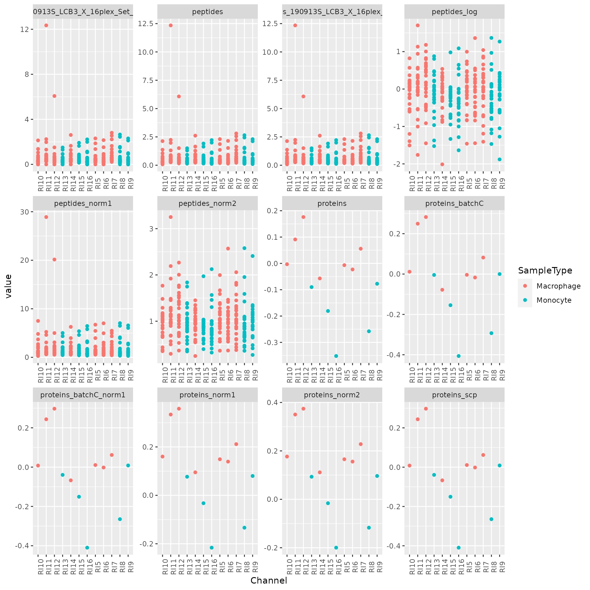
This graph can be used to track the processing of the quantitative data.
Since each assay is a SingleCellExperiment object, the data can also easily be plugged into dimension reduction functions from the Bioconductor package scater. We show here an example of dimension reduction results using t-SNE.
sce <- getWithColData(lcb3, "proteins_scp")
## Warning: 'experiments' dropped; see 'metadata'
## Warning: Ignoring redundant column names in 'colData(x)':
library(scater)
set.seed(1234)
sce <- runTSNE(sce,
               ncomponents = 2,
               ntop = Inf,
               scale = TRUE,
               exprs_values = 1,
               name = "TSNE")
## Plotting is performed in a single line of code
plotTSNE(sce, colour_by = "SampleType")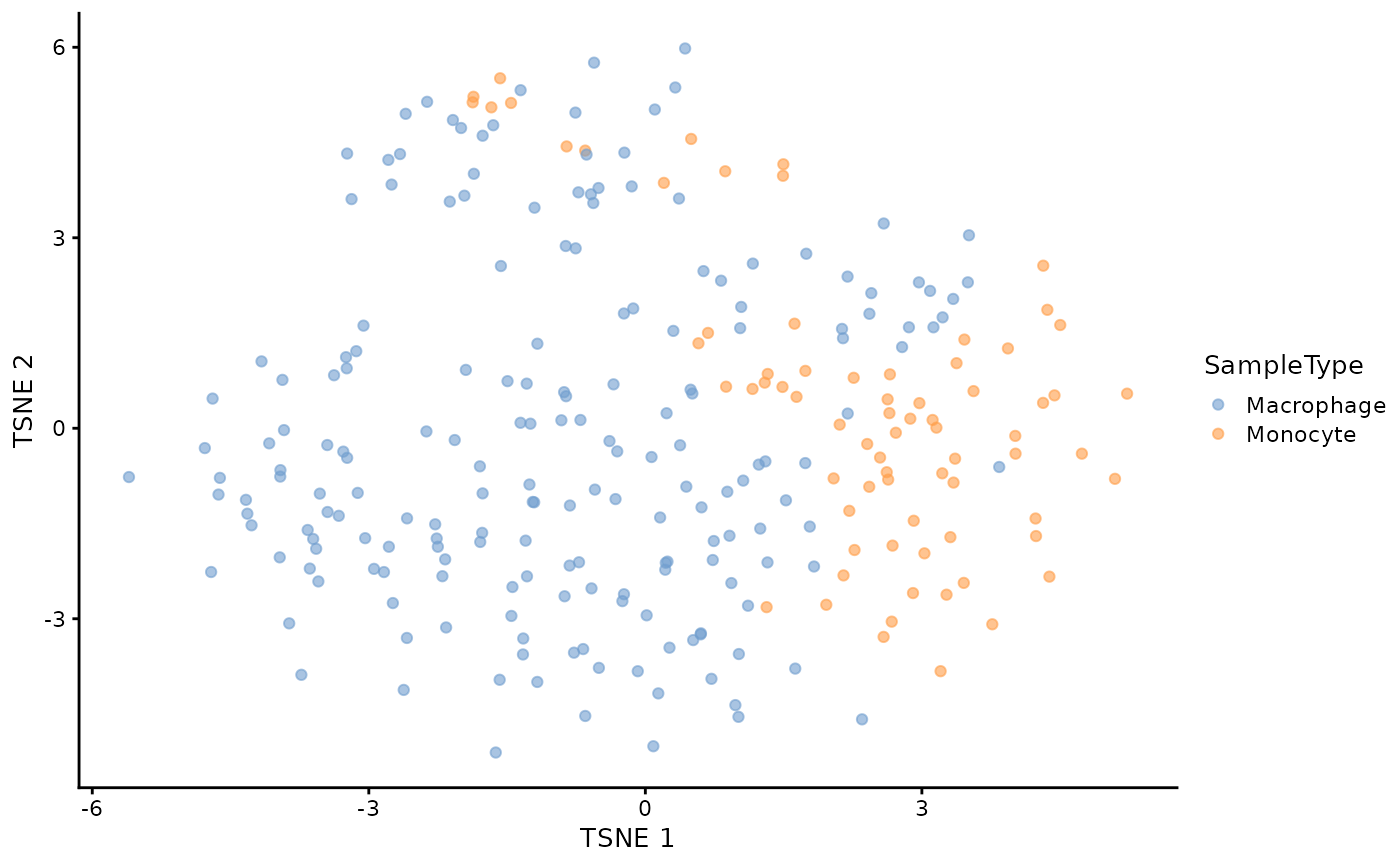
This graph shows a low dimension representation of the final processed protein data. Each point represents a cell. The sample type is accessed from the colData and coloured on the graph. This allows to evaluate whether the quantitative data contains information to separate monocytes from differentiated macrophages.
Conclusion
We hope we could convince you that QFeatures and its extension scp are an ideal environment to manipulate and process MS-SCP quantification data. This is only the beginning of the journey, as further development and benchmarking are required to offer improved processing workflows. Furthermore, downstream analyses, such as differential expression analyses, require the development of new statistical methods to model the complex data structure present in SCP data (Vanderaa and Gatto (2021)). Those methods could highly benefit from the QFeatures and scp infrastructure to access and manipulate the required information. Furthermore, the scpdata package provides ready-to-process data that represent valuable use cases to build analytical method onto.
Further reading
- You can find more information about how to load your own data using
scpin this vignette. - We also dedicated a separate vignette about data visualization from a
QFeaturesobject. - If you want to push forward the development of new analytical methods and QC metrics in for single-cell proteomics, we also recommend you to read the advanced vignette.
Have a look at our paper that describes the reproduction of the complete SCoPE2 data set and highlights some important challenges that remain to be tackled in the field.
Session information
sessionInfo()
## R version 4.1.0 (2021-05-18)
## Platform: x86_64-pc-linux-gnu (64-bit)
## Running under: Ubuntu 20.04.2 LTS
##
## Matrix products: default
## BLAS/LAPACK: /usr/lib/x86_64-linux-gnu/openblas-pthread/libopenblasp-r0.3.8.so
##
## locale:
##  [1] LC_CTYPE=en_US.UTF-8       LC_NUMERIC=C
##  [3] LC_TIME=en_US.UTF-8        LC_COLLATE=en_US.UTF-8
##  [5] LC_MONETARY=en_US.UTF-8    LC_MESSAGES=C
##  [7] LC_PAPER=en_US.UTF-8       LC_NAME=C
##  [9] LC_ADDRESS=C               LC_TELEPHONE=C
## [11] LC_MEASUREMENT=en_US.UTF-8 LC_IDENTIFICATION=C
##
## attached base packages:
## [1] stats4    stats     graphics  grDevices utils     datasets  methods
## [8] base
##
## other attached packages:
##  [1] scater_1.21.3               scuttle_1.3.1
##  [3] SingleCellExperiment_1.15.1 forcats_0.5.1
##  [5] stringr_1.4.0               dplyr_1.0.7
##  [7] purrr_0.3.4                 readr_2.0.1
##  [9] tidyr_1.1.3                 tibble_3.1.3
## [11] ggplot2_3.3.5               tidyverse_1.3.1
## [13] sva_3.41.0                  BiocParallel_1.27.3
## [15] genefilter_1.75.0           mgcv_1.8-36
## [17] nlme_3.1-152                scpdata_1.1.0
## [19] ExperimentHub_2.1.4         AnnotationHub_3.1.4
## [21] BiocFileCache_2.1.1         dbplyr_2.1.1
## [23] scp_1.3.3                   QFeatures_1.3.7
## [25] MultiAssayExperiment_1.19.5 SummarizedExperiment_1.23.1
## [27] Biobase_2.53.0              GenomicRanges_1.45.0
## [29] GenomeInfoDb_1.29.3         IRanges_2.27.0
## [31] S4Vectors_0.31.0            BiocGenerics_0.39.1
## [33] MatrixGenerics_1.5.3        matrixStats_0.60.0
## [35] BiocStyle_2.21.3
##
## loaded via a namespace (and not attached):
##   [1] readxl_1.3.1                  backports_1.2.1
##   [3] systemfonts_1.0.2             igraph_1.2.6
##   [5] lazyeval_0.2.2                splines_4.1.0
##   [7] digest_0.6.27                 htmltools_0.5.1.1
##   [9] viridis_0.6.1                 fansi_0.5.0
##  [11] magrittr_2.0.1                memoise_2.0.0
##  [13] ScaledMatrix_1.1.0            cluster_2.1.2
##  [15] tzdb_0.1.2                    limma_3.49.4
##  [17] Biostrings_2.61.2             annotate_1.71.0
##  [19] modelr_0.1.8                  pkgdown_1.6.1
##  [21] colorspace_2.0-2              ggrepel_0.9.1
##  [23] blob_1.2.2                    rvest_1.0.1
##  [25] rappdirs_0.3.3                textshaping_0.3.5
##  [27] haven_2.4.3                   xfun_0.25
##  [29] crayon_1.4.1                  RCurl_1.98-1.3
##  [31] jsonlite_1.7.2                impute_1.67.0
##  [33] survival_3.2-11               glue_1.4.2
##  [35] gtable_0.3.0                  zlibbioc_1.39.0
##  [37] XVector_0.33.0                DelayedArray_0.19.1
##  [39] BiocSingular_1.9.1            scales_1.1.1
##  [41] DBI_1.1.1                     edgeR_3.35.0
##  [43] Rcpp_1.0.7                    viridisLite_0.4.0
##  [45] xtable_1.8-4                  clue_0.3-59
##  [47] rsvd_1.0.5                    bit_4.0.4
##  [49] MsCoreUtils_1.5.0             httr_1.4.2
##  [51] ellipsis_0.3.2                farver_2.1.0
##  [53] pkgconfig_2.0.3               XML_3.99-0.6
##  [55] sass_0.4.0                    locfit_1.5-9.4
##  [57] utf8_1.2.2                    labeling_0.4.2
##  [59] tidyselect_1.1.1              rlang_0.4.11
##  [61] later_1.2.0                   AnnotationDbi_1.55.1
##  [63] munsell_0.5.0                 BiocVersion_3.14.0
##  [65] cellranger_1.1.0              tools_4.1.0
##  [67] cachem_1.0.5                  cli_3.0.1
##  [69] generics_0.1.0                RSQLite_2.2.7
##  [71] broom_0.7.9                   evaluate_0.14
##  [73] fastmap_1.1.0                 yaml_2.2.1
##  [75] ragg_1.1.3                    knitr_1.33
##  [77] bit64_4.0.5                   fs_1.5.0
##  [79] KEGGREST_1.33.0               AnnotationFilter_1.17.1
##  [81] sparseMatrixStats_1.5.2       mime_0.11
##  [83] xml2_1.3.2                    compiler_4.1.0
##  [85] rstudioapi_0.13               beeswarm_0.4.0
##  [87] filelock_1.0.2                curl_4.3.2
##  [89] png_0.1-7                     interactiveDisplayBase_1.31.2
##  [91] reprex_2.0.1                  bslib_0.2.5.1
##  [93] stringi_1.7.3                 highr_0.9
##  [95] desc_1.3.0                    lattice_0.20-44
##  [97] ProtGenerics_1.25.1           Matrix_1.3-4
##  [99] vctrs_0.3.8                   pillar_1.6.2
## [101] lifecycle_1.0.0               BiocManager_1.30.16
## [103] jquerylib_0.1.4               BiocNeighbors_1.11.0
## [105] cowplot_1.1.1                 irlba_2.3.3
## [107] bitops_1.0-7                  httpuv_1.6.1
## [109] R6_2.5.0                      promises_1.2.0.1
## [111] gridExtra_2.3                 vipor_0.4.5
## [113] MASS_7.3-54                   assertthat_0.2.1
## [115] rprojroot_2.0.2               withr_2.4.2
## [117] GenomeInfoDbData_1.2.6        parallel_4.1.0
## [119] hms_1.1.0                     beachmat_2.9.0
## [121] grid_4.1.0                    DelayedMatrixStats_1.15.2
## [123] rmarkdown_2.10                Rtsne_0.15
## [125] shiny_1.6.0                   lubridate_1.7.10
## [127] ggbeeswarm_0.6.0