Quantitative proteomics data analysis with QFeatures
Laurent Gatto and Christophe Vanderaa
Source:vignettes/v02-QFeaturesPipeline.Rmd
v02-QFeaturesPipeline.RmdLast modified: NA
Compiled: Tue Dec 15 15:52:48 2020
Learning Objectives The goals of this workshop are to provide a real-life example of step-by-step quantitative proteomics data analysis using the QFeatures package. This vignette demonstrates an application using spiked-in data.
Analysis pipeline
Quantitative proteomics data processing is composed of the following steps:
- Data import
- Exploratory data analysis (PCA)
- Missing data management (filtering and/or imputation)
- Data cleaning
- Transformation and normalisation
- Aggregation
- Downstream analysis
Let’s start by loading the requried packages
The CPTAC data
The CPTAC spike-in study 6 (Paulovich et al. 2010) combines the Sigma UPS1 standard containing 48 different human proteins that are spiked in at 5 different concentrations (conditions A to E) into a constant yeast protein background. The sample were acquired in triplicate on different instruments in different labs. We are going to start with a subset of the CPTAC study 6 containing conditions A and B for a single lab.
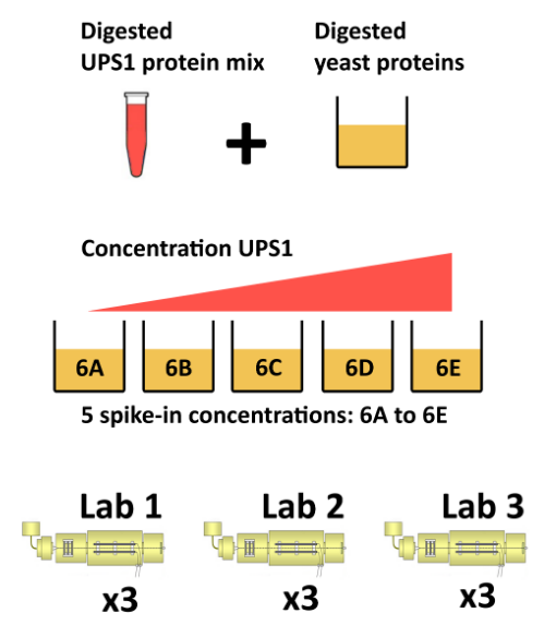
The CPTAC spike-in study design (credit Lieven Clement, statOmics, Ghent University).
The peptide-level data, as processed by MaxQuant (Cox and Mann 2008) is available in the msdata package:
From the names of the columns, we see that the quantitative columns, starting with "Intensity." (note the dot!) are at positions 56 to 61.
names(read.delim(f))
##  [1] "Sequence"                 "N.term.cleavage.window"
##  [3] "C.term.cleavage.window"   "Amino.acid.before"
##  [5] "First.amino.acid"         "Second.amino.acid"
##  [7] "Second.last.amino.acid"   "Last.amino.acid"
##  [9] "Amino.acid.after"         "A.Count"
## [11] "R.Count"                  "N.Count"
## [13] "D.Count"                  "C.Count"
## [15] "Q.Count"                  "E.Count"
## [17] "G.Count"                  "H.Count"
## [19] "I.Count"                  "L.Count"
## [21] "K.Count"                  "M.Count"
## [23] "F.Count"                  "P.Count"
## [25] "S.Count"                  "T.Count"
## [27] "W.Count"                  "Y.Count"
## [29] "V.Count"                  "U.Count"
## [31] "Length"                   "Missed.cleavages"
## [33] "Mass"                     "Proteins"
## [35] "Leading.razor.protein"    "Start.position"
## [37] "End.position"             "Unique..Groups."
## [39] "Unique..Proteins."        "Charges"
## [41] "PEP"                      "Score"
## [43] "Identification.type.6A_7" "Identification.type.6A_8"
## [45] "Identification.type.6A_9" "Identification.type.6B_7"
## [47] "Identification.type.6B_8" "Identification.type.6B_9"
## [49] "Experiment.6A_7"          "Experiment.6A_8"
## [51] "Experiment.6A_9"          "Experiment.6B_7"
## [53] "Experiment.6B_8"          "Experiment.6B_9"
## [55] "Intensity"                "Intensity.6A_7"
## [57] "Intensity.6A_8"           "Intensity.6A_9"
## [59] "Intensity.6B_7"           "Intensity.6B_8"
## [61] "Intensity.6B_9"           "Reverse"
## [63] "Potential.contaminant"    "id"
## [65] "Protein.group.IDs"        "Mod..peptide.IDs"
## [67] "Evidence.IDs"             "MS.MS.IDs"
## [69] "Best.MS.MS"               "Oxidation..M..site.IDs"
## [71] "MS.MS.Count"
(i <- grep("Intensity\\.", names(read.delim(f))))
## [1] 56 57 58 59 60 61
We now read these data using the readSummarizedExperiment function. This peptide-level expression data will be imported into R as an instance of class SummarizedExperiment. We also use the fnames argument to set the row-names of the peptides assay to the peptide sequences and specify that the file is a tab-separated table.
cptac_se <- readSummarizedExperiment(f, ecol = i, fnames = "Sequence", sep = "\t")
cptac_se
## class: SummarizedExperiment
## dim: 11466 6
## metadata(0):
## assays(1): ''
## rownames(11466): AAAAGAGGAGDSGDAVTK AAAALAGGK ... YYTVFDRDNNR
##   YYTVFDRDNNRVGFAEAAR
## rowData names(65): Sequence N.term.cleavage.window ...
##   Oxidation..M..site.IDs MS.MS.Count
## colnames(6): Intensity.6A_7 Intensity.6A_8 ... Intensity.6B_8
##   Intensity.6B_9
## colData names(0):
Before proceeding, we are going to clean up the sample names and annotate the experiment:
colnames(cptac_se) <- sub("I.+\\.", "", colnames(cptac_se))
cptac_se$condition <- sub("_[7-9]", "", colnames(cptac_se))
cptac_se$id <- sub("^.+_", "", colnames(cptac_se))
colData(cptac_se)
## DataFrame with 6 rows and 2 columns
##        condition          id
##      <character> <character>
## 6A_7          6A           7
## 6A_8          6A           8
## 6A_9          6A           9
## 6B_7          6B           7
## 6B_8          6B           8
## 6B_9          6B           9
Let’s also keep only a subset of
keep_var <- c("Sequence", "Proteins", "Leading.razor.protein", "PEP",
              "Score", "Reverse", "Potential.contaminant")

rowData(cptac_se) <- rowData(cptac_se)[, keep_var]
Missing values
Missing values can be highly frequent in proteomics. These exist two reasons supporting the existence of missing values, namely biological or technical.
Values that are missing due to the absence (or extremely low contentration) of a protein are observed for biological reasons, and their pattern aren’t random. A protein missing in due to the suppression of its expression will not be missing at random: it will be missing in the condition in which it was suppressed, and be present in the condition where it is expressed.
Due to it’s data-dependent acquisition, mass spectrometry isn’t capable to assaying all peptides in a sample. Peptides that are less abundant than some of their co-eluting ions, peptides that do not ionise well or peptides that do not get identified might be sporadically missing in the final quantitation table, despite their presence in the biological samples. Their absence patterns are random in such cases.
Often, third party software that produce quantiative data use zeros instead of properly reporting missing values. We can use the zeroIsNA() function to replace the 0 by NA values in our cptac_se object and then explore the missing data patterns across columns and rows.
cptac_se <- zeroIsNA(cptac_se)
nNA(cptac_se)
## $nNA
## DataFrame with 1 row and 2 columns
##         nNA       pNA
##   <integer> <numeric>
## 1     31130   45.2497
##
## $nNArows
## DataFrame with 11466 rows and 3 columns
##                name       nNA       pNA
##         <character> <integer> <numeric>
## 1     AAAAGAGGAG...         4   66.6667
## 2         AAAALAGGK         0    0.0000
## 3        AAAALAGGKK         0    0.0000
## 4     AAADALSDLE...         0    0.0000
## 5     AAADALSDLE...         0    0.0000
## ...             ...       ...       ...
## 11462 YYSIYDLGNN...         6  100.0000
## 11463 YYTFNGPNYN...         3   50.0000
## 11464    YYTITEVATR         4   66.6667
## 11465 YYTVFDRDNN...         6  100.0000
## 11466 YYTVFDRDNN...         6  100.0000
##
## $nNAcols
## DataFrame with 6 rows and 3 columns
##          name       nNA       pNA
##   <character> <integer> <numeric>
## 1        6A_7      4743   41.3658
## 2        6A_8      5483   47.8196
## 3        6A_9      5320   46.3980
## 4        6B_7      4721   41.1739
## 5        6B_8      5563   48.5174
## 6        6B_9      5300   46.2236
Distribution of missing value (white). Peptides row with more missing values are moved towards the top of the figure.
Let’s now explore these missing values:
- Explore the number or proportion of missing values across peptides and samples of the
cptac_sedata.

- Remove row that have too many missing values. You can do this by hand or using the
filterNA()function.
## remove rows that have 4 or more NAs out of 6
cptac_se <- filterNA(cptac_se, pNA = 4/6)
Imputation
Imputation is the technique of replacing missing data with probable values. This can be done with impute() method. As we have discussed above, there are however two types of missing values in mass spectrometry-based proteomics, namely data missing at random (MAR), and data missing not at random (MNAR). These two types of missing data need to be imputed with different types of imputation methods (Lazar et al. 2016).
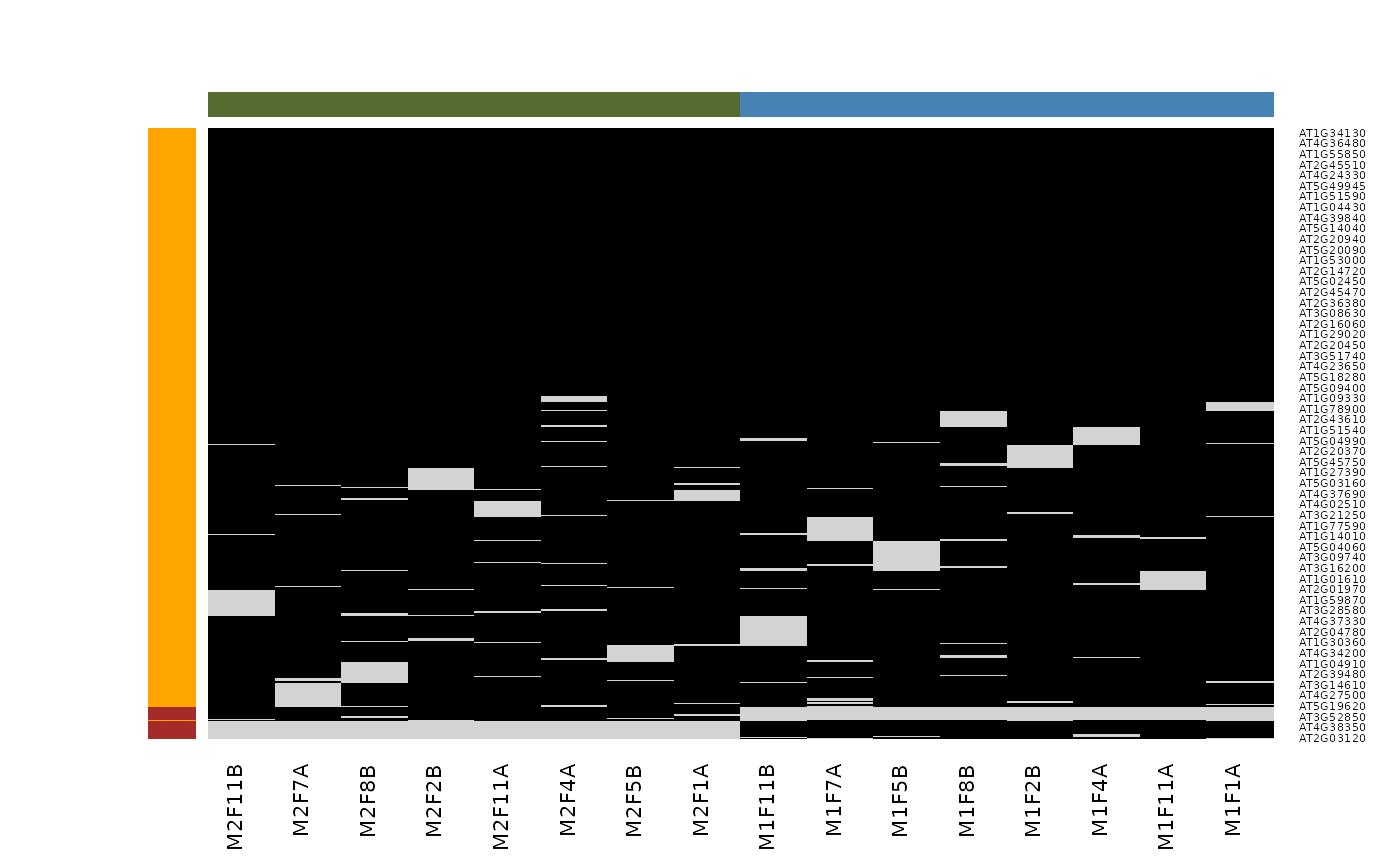
Mixed imputation method. Black cells represent presence of quantitation values and light grey corresponds to missing data. The two groups of interest are depicted in green and blue along the heatmap columns. Two classes of proteins are annotated on the left: yellow are proteins with randomly occurring missing values (if any) while proteins in brown are candidates for non-random missing value imputation.
When downstream analyses permit, it might thus be safer not to impute data and deal explicitly with missing values. This is possible when performing hypethesis tests, but not to perform a principal component analysis.
Identification quality control
As discussed in the previous chapter, PSMs are deemed relevant after comparison against hist from a decoy database. The origin of these hits is recorded with + in the Reverse variable:
table(rowData(cptac_se)$Reverse)
##
##         +
## 7572   12
Similarly, a proteomics experiment is also searched against a database of contaminants:
table(rowData(cptac_se)$Potential.contaminant)
##
##         +
## 7558   26
Let’s visualise some of the cptac’s metadata using standard ggplot2 code:
- Visualise the score distributions from forward and reverse hits and interpret the figure.
rowData(cptac_se) %>%
    as_tibble() %>%
    ggplot(aes(x = Score, colour = Reverse)) +
    geom_density()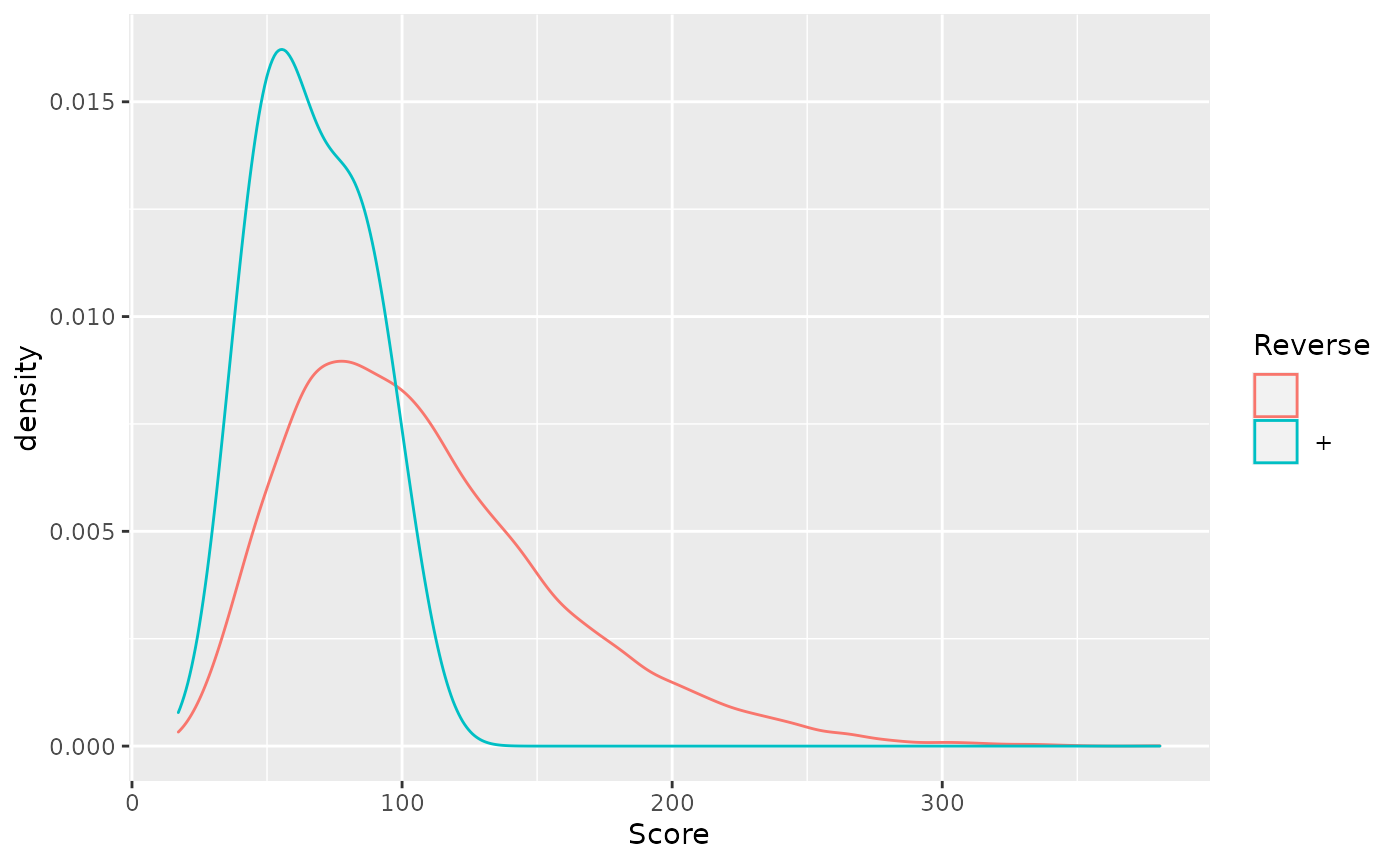
- Do the same with the posterior probability score (PEP).
rowData(cptac_se) %>%
    as_tibble() %>%
    ggplot(aes(x = PEP, colour = Reverse)) +
    geom_density()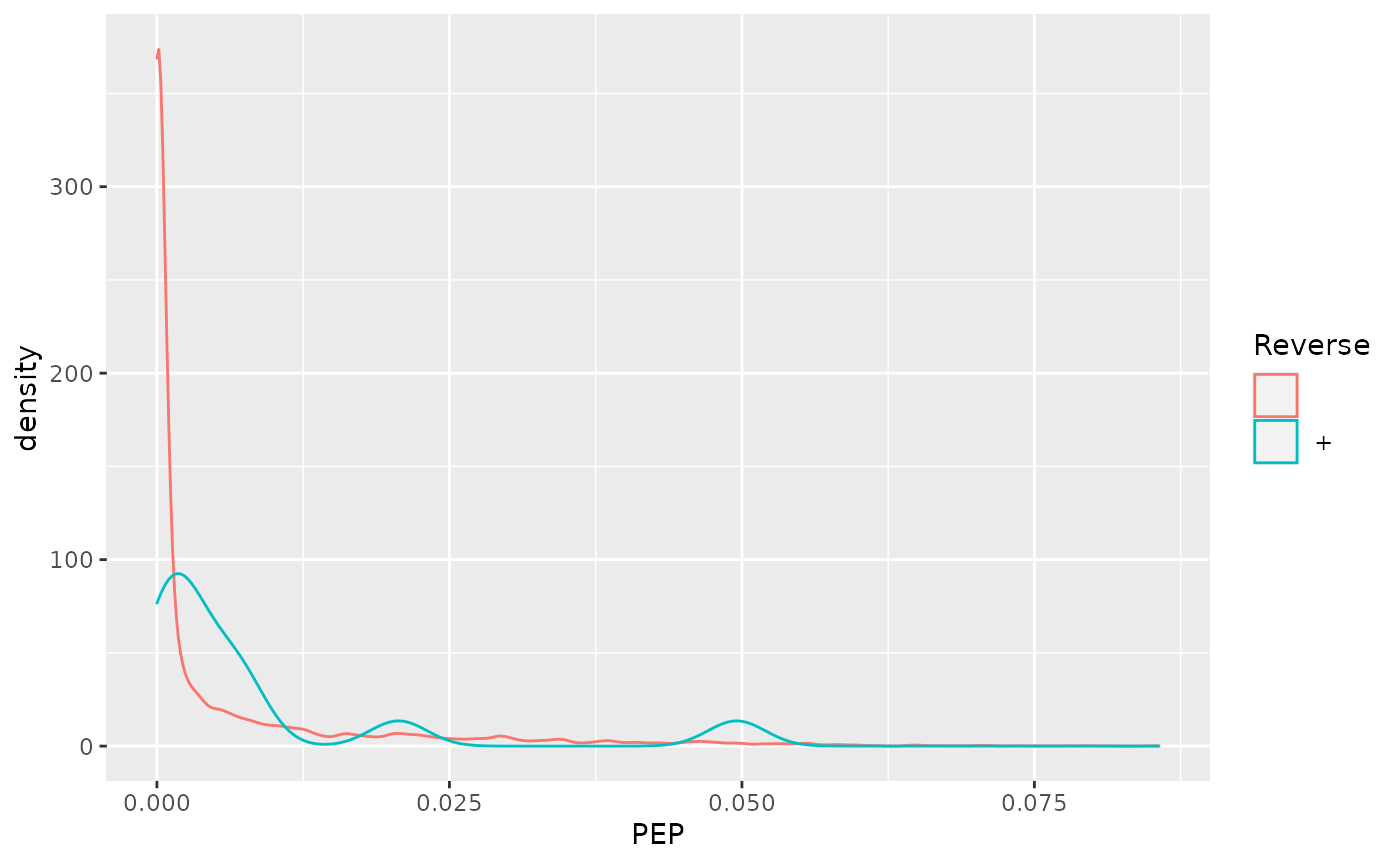
Creating the QFeatures data
We can now create our QFeatures object using the SummarizedExperiment as show below.
cptac <- QFeatures(list(peptides = cptac_se))
cptac
## An instance of class QFeatures containing 1 assays:
##  [1] peptides: SummarizedExperiment with 7584 rows and 6 columns
We should also assign the QFeatures column data with the SummarizedExperiment slot.
colData(cptac) <- colData(cptac_se)Note that it is also possible to directly create a QFeatures object with the readQFeatures() function and the same arguments as the readSummarizedExperiment() used above. In addition, most functions used above and below work on single SummarizedExperiment objects or assays within a QFeatures object.
Filtering out contaminants and reverse hits
Using the filterFeatures() function, filter out the reverse and contaminant hits.
cptac <-
    cptac %>%
    filterFeatures(~ Reverse != "+") %>%
    filterFeatures(~ Potential.contaminant != "+")
Log-transformation and normaliation
The two code chunks below log-transform and normalise using the assay i as input and adding a new one names as defined by name.
cptac <- logTransform(cptac, i = "peptides",
                      name = "log_peptides")
cptac <- normalize(cptac, i = "log_peptides",
                   name = "lognorm_peptides",
                   method = "center.median")
par(mfrow = c(1, 3))
limma::plotDensities(assay(cptac[["peptides"]]))
limma::plotDensities(assay(cptac[["log_peptides"]]))
limma::plotDensities(assay(cptac[["lognorm_peptides"]]))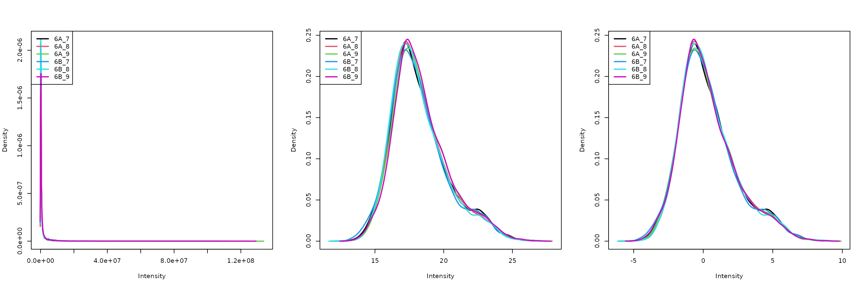
Three peptide level assays: raw data, log transformed and normalised.
Aggregation
Below, we are going to use median aggregation, as a first attempt. This is however not the best choice, as we will see later.
cptac <-
    aggregateFeatures(cptac,
                      "lognorm_peptides",
                      name = "proteins_med",
                      fcol = "Leading.razor.protein",
                      fun = colMedians,
                      na.rm = TRUE)
Looking at the .n row variable computed during the aggregation, we see that most proteins result of the aggregation of 5 peptides or less, while very few proteins are accounted for by tens of peptides.
table(rowData(cptac[["proteins_med"]])$.n)
##
##   1   2   3   4   5   6   7   8   9  10  11  12  13  14  15  16  17  18  19  20
## 328 234 162 138  85  72  66  49  46  34  25  28  21  12  17   9   5   4  13   5
##  21  22  23  24  25  26  28  29  30  31  32  35  38  39  42  43  51  52  62
##   7   6   4   4   3   3   1   3   1   1   3   1   2   1   1   1   1   1   1
Principal component analysis
library("factoextra")
library("patchwork")

pca_pep <-
    cptac[["lognorm_peptides"]] %>%
    filterNA() %>%
    assay() %>%
    t() %>%
    prcomp(scale = TRUE, center = TRUE) %>%
    fviz_pca_ind(habillage = cptac$condition, title = "Peptides")

pca_prot <-
    cptac[["proteins_med"]] %>%
    filterNA() %>%
    assay() %>%
    t() %>%
    prcomp() %>%
    fviz_pca_ind(habillage = cptac$condition,
                 title = "Proteins (median aggregation)")
pca_pep + pca_prot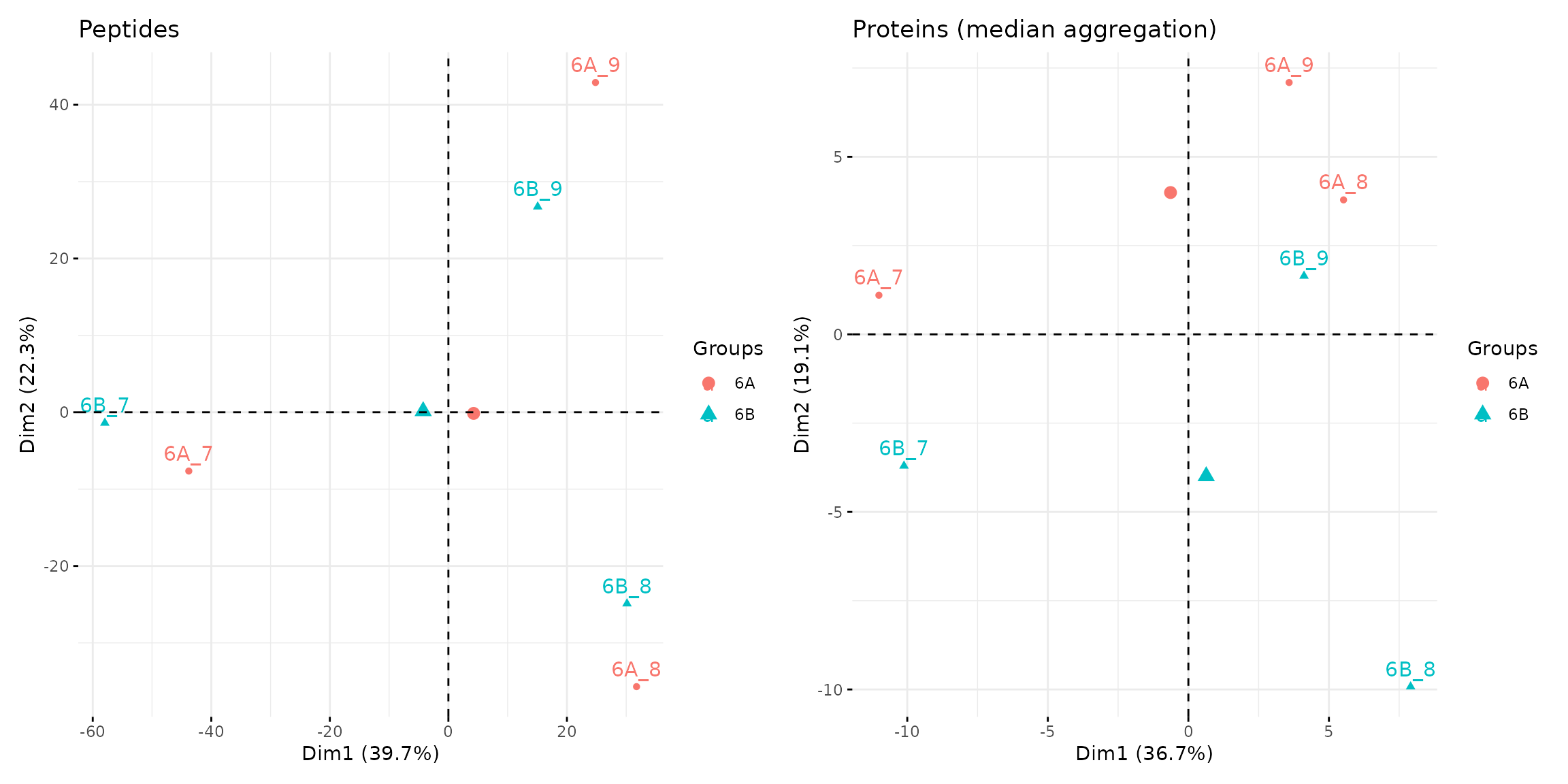
Peptide and protein level PCA analyses.
Visualisation
Below, we use the longFormat() function to extract the quantitative and row data in a long format, that can be directly reused by the tidyverse tools.
longFormat(cptac["P02787ups|TRFE_HUMAN_UPS", ,
                 c("lognorm_peptides", "proteins_med")]) %>%
    as_tibble() %>%
    mutate(condition = ifelse(grepl("A", colname), "A", "B")) %>%
    ggplot(aes(x = colname, y = value, colour = rowname, shape = condition)) +
    geom_point(size = 3) +
    geom_line(aes(group = rowname)) +
    facet_grid(~ assay) +
    ggtitle("P02787ups|TRFE_HUMAN_UPS")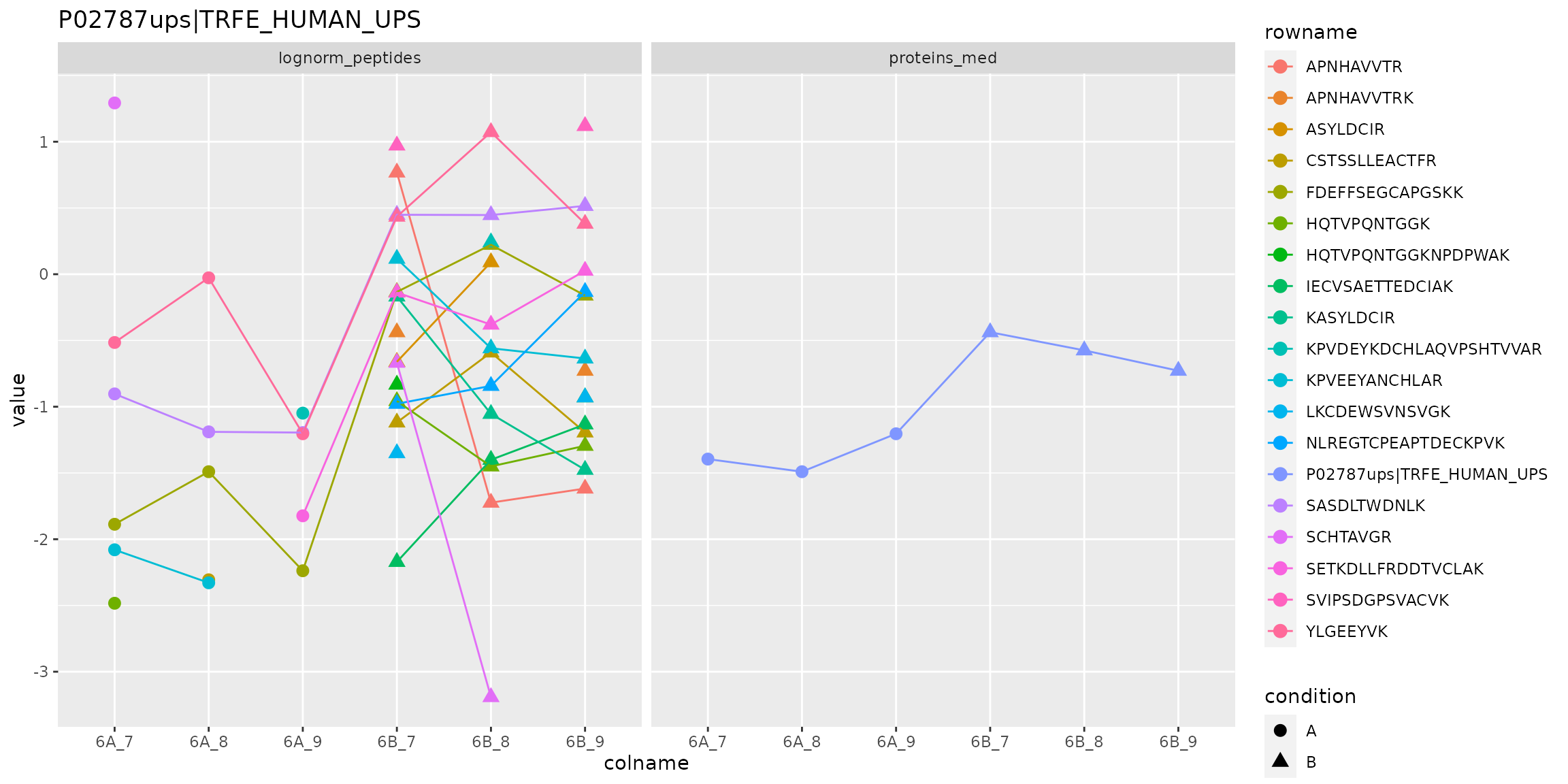
Peptide and protein expression profile.
Statistical analysis
Below, we are going to perform our statistical analysis on the protein data.
prots <- cptac[["proteins_med"]]
colData(prots) <- colData(cptac)
The limma package is the precursor package that enables the consistent application of linear models to normalliy distributed omics data in general, and microarrays in particuar.
The limma package implements an empirical Bayes method that provides borrows information across features to estimate the standard error and calculate (so called moderate) t statistics. This approach is demonstrably more powerful that a standard t-tests when the number of samples is lot.
The code chunk below illstrated how to set up the model, fit it, and apply the empirical Bayes moderation.
library("limma")
design <- model.matrix(~ prots$condition)
fit <- lmFit(assay(prots), design)
## Warning: Partial NA coefficients for 23 probe(s)
fit <- eBayes(fit)
Finally, the topTable() function is used the extract the results for the coefficient of interest.
res <-
    topTable(fit, coef = "prots$condition6B", number = Inf) %>%
    rownames_to_column("protein") %>%
    as_tibble() %>%
    mutate(TP = grepl("ups", protein))
Note the warning about partial NA coefficients for 23 probes:
na_coefs <-
filter(res, is.na(t)) %>%
pull(protein)
assay(prots[na_coefs, ])
## 6A_7 6A_8 6A_9 6B_7 6B_8
## P00167ups|CYB5_HUMAN_UPS NaN NaN NaN -0.7642817 -2.0050174
## P01112ups|RASH_HUMAN_UPS NaN NaN NaN -1.5367155 NaN
## P05413ups|FABPH_HUMAN_UPS NaN NaN NaN -3.3221739 NaN
## P08758ups|ANXA5_HUMAN_UPS NaN NaN NaN -2.7776131 -1.9904771
## sp|P06704|CDC31_YEAST NaN NaN NaN -1.1834305 -2.1019557
## sp|P32608|RTG2_YEAST NaN NaN NaN NaN -4.4191375
## sp|P32769|HBS1_YEAST NaN -1.359851 -0.7138411 NaN NaN
## sp|P34217|PIN4_YEAST NaN NaN NaN -0.8180873 -0.1083583
## sp|P34237|CASP_YEAST NaN NaN NaN -1.5447431 -1.6367477
## sp|P38166|SFT2_YEAST -1.564052 -1.052527 NaN NaN NaN
## sp|P40056|GET2_YEAST NaN -1.067516 -1.3866843 NaN NaN
## sp|P40533|TED1_YEAST NaN NaN NaN -2.0294135 NaN
## sp|P46965|SPC1_YEAST NaN -3.404591 -3.6174615 NaN NaN
## sp|P48363|PFD3_YEAST NaN NaN NaN -0.1707164 NaN
## sp|P53044|UFD1_YEAST NaN NaN NaN -2.3740155 -1.4905932
## sp|P53091|MCM6_YEAST NaN -1.229600 -1.6762933 NaN NaN
## sp|P53115|INO80_YEAST NaN NaN NaN -2.6986219 NaN
## sp|P53893|RIA1_YEAST -1.809222 NaN -1.5085444 NaN NaN
## sp|Q05029|BCH1_YEAST -1.836222 -1.736322 NaN NaN NaN
## sp|Q07540|FRDA_YEAST NaN NaN NaN -2.3652501 NaN
## sp|Q08645|FOLE_YEAST NaN NaN NaN -1.7071443 NaN
## sp|Q12255|NYV1_YEAST NaN NaN NaN -2.8508289 NaN
## sp|Q12280|IQG1_YEAST NaN NaN NaN -2.5438648 -2.0314751
## 6B_9
## P00167ups|CYB5_HUMAN_UPS -1.1067954
## P01112ups|RASH_HUMAN_UPS -1.5455337
## P05413ups|FABPH_HUMAN_UPS -3.8744226
## P08758ups|ANXA5_HUMAN_UPS -2.0731897
## sp|P06704|CDC31_YEAST -1.5681249
## sp|P32608|RTG2_YEAST -2.7710331
## sp|P32769|HBS1_YEAST NaN
## sp|P34217|PIN4_YEAST -0.1826536
## sp|P34237|CASP_YEAST -1.6714608
## sp|P38166|SFT2_YEAST NaN
## sp|P40056|GET2_YEAST NaN
## sp|P40533|TED1_YEAST -1.7311957
## sp|P46965|SPC1_YEAST NaN
## sp|P48363|PFD3_YEAST -0.4924892
## sp|P53044|UFD1_YEAST NaN
## sp|P53091|MCM6_YEAST NaN
## sp|P53115|INO80_YEAST -2.7341224
## sp|P53893|RIA1_YEAST NaN
## sp|Q05029|BCH1_YEAST NaN
## sp|Q07540|FRDA_YEAST -2.0162325
## sp|Q08645|FOLE_YEAST -1.5094503
## sp|Q12255|NYV1_YEAST -2.8074462
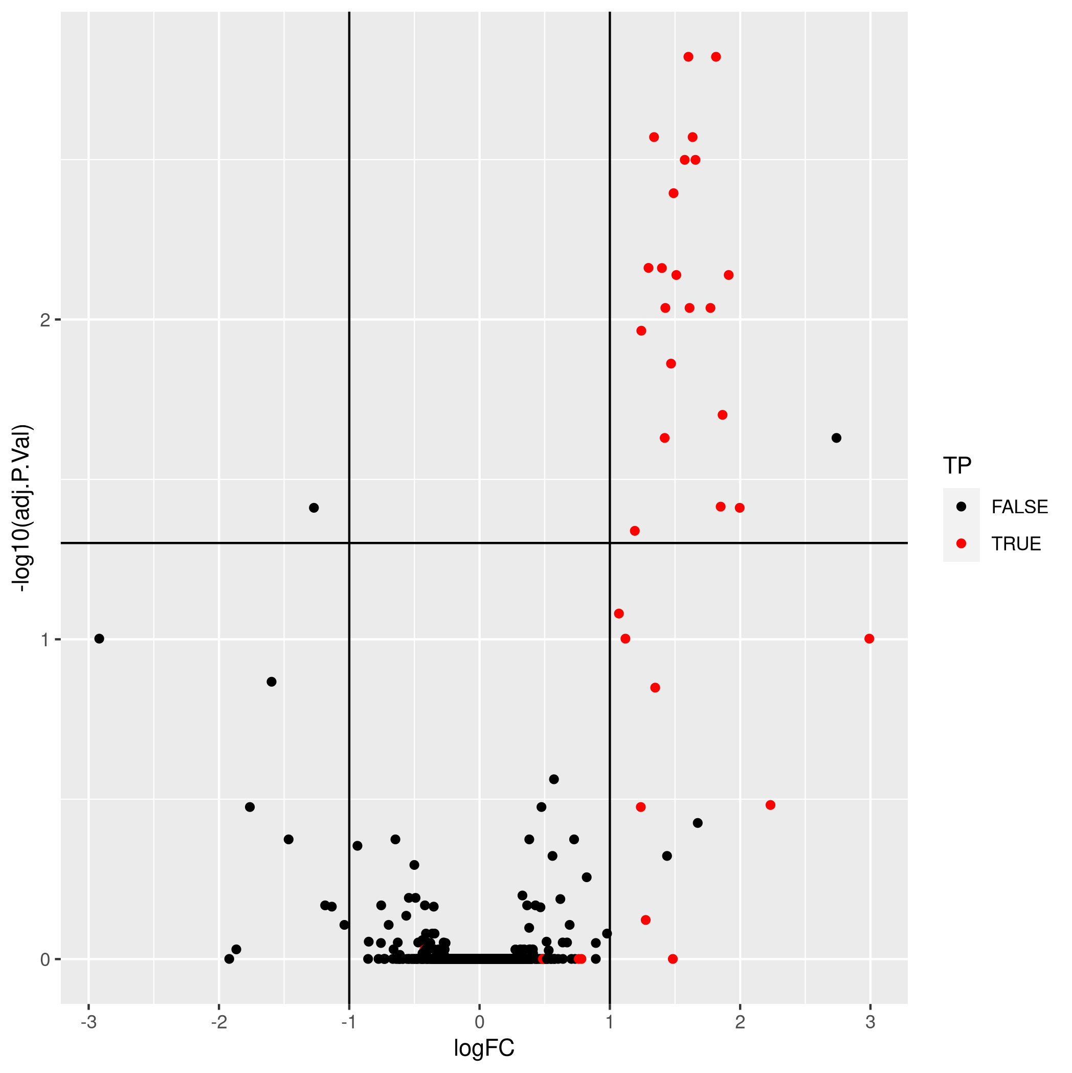
## sp|Q12280|IQG1_YEAST -2.4485187We can now visualise the results using a volcano plot:
res %>%
    ggplot(aes(x = logFC, y = -log10(adj.P.Val))) +
    geom_point(aes(colour = TP)) +
    geom_vline(xintercept = c(-1, 1)) +
    geom_hline(yintercept = -log10(0.05)) +
    scale_color_manual(values = c("black","red"))
## Warning: Removed 23 rows containing missing values (geom_point).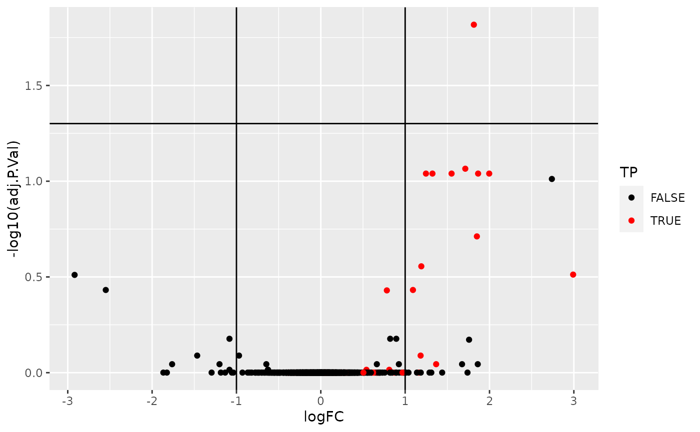
Volcano plot highlighing spiked-in proteins in red.
Using the pipeline described above, we would would identify a single differentially expressed protein at an 5 percent FDR but miss out the other 36 expected spike-in proteins.
We can assess our results in terms of true/false postitves/negatives:
- True positives: 1
- False positives: 0
- True negatives: 1342
- False negatives: 32
Final exercise
As shown below, it is possible to substantially improve these results by aggregating features using a robust summarisation (available as MsCoreUtils::robustSummary()), i.e robust regression with M-estimation using Huber weights, as described in section 2.7 in (Sticker et al. 2019).
Aggregation using robust summarisation.
- True positives: 21
- False positives: 2
- True negatives: 1340
- False negatives: 12
Repeat and adapt what we have seen here using, for example, the robustSummary() function.
Session information
sessionInfo()
## R Under development (unstable) (2020-11-02 r79396)
## Platform: x86_64-pc-linux-gnu (64-bit)
## Running under: Ubuntu 20.04.1 LTS
##
## Matrix products: default
## BLAS/LAPACK: /usr/lib/x86_64-linux-gnu/openblas-pthread/libopenblasp-r0.3.8.so
##
## locale:
##  [1] LC_CTYPE=en_US.UTF-8       LC_NUMERIC=C
##  [3] LC_TIME=en_US.UTF-8        LC_COLLATE=en_US.UTF-8
##  [5] LC_MONETARY=en_US.UTF-8    LC_MESSAGES=C
##  [7] LC_PAPER=en_US.UTF-8       LC_NAME=C
##  [9] LC_ADDRESS=C               LC_TELEPHONE=C
## [11] LC_MEASUREMENT=en_US.UTF-8 LC_IDENTIFICATION=C
##
## attached base packages:
## [1] parallel  stats4    stats     graphics  grDevices utils     datasets
## [8] methods   base
##
## other attached packages:
##  [1] patchwork_1.1.0             factoextra_1.0.7
##  [3] gplots_3.1.1                limma_3.47.1
##  [5] QFeatures_1.1.0             MultiAssayExperiment_1.17.2
##  [7] SummarizedExperiment_1.21.1 Biobase_2.51.0
##  [9] GenomicRanges_1.43.1        GenomeInfoDb_1.27.3
## [11] IRanges_2.25.5              S4Vectors_0.29.6
## [13] BiocGenerics_0.37.0         MatrixGenerics_1.3.0
## [15] matrixStats_0.57.0          forcats_0.5.0
## [17] stringr_1.4.0               dplyr_1.0.2
## [19] purrr_0.3.4                 readr_1.4.0
## [21] tidyr_1.1.2                 tibble_3.0.4
## [23] ggplot2_3.3.2               tidyverse_1.3.0
## [25] BiocStyle_2.19.1
##
## loaded via a namespace (and not attached):
##  [1] colorspace_2.0-0        ggsignif_0.6.0          ellipsis_0.3.1
##  [4] rio_0.5.16              rprojroot_2.0.2         XVector_0.31.1
##  [7] fs_1.5.0                rstudioapi_0.13         ggpubr_0.4.0
## [10] farver_2.0.3            ggrepel_0.8.2           fansi_0.4.1
## [13] lubridate_1.7.9.2       xml2_1.3.2              knitr_1.30
## [16] jsonlite_1.7.2          broom_0.7.2             dbplyr_2.0.0
## [19] BiocManager_1.30.10     compiler_4.1.0          httr_1.4.2
## [22] backports_1.2.1         assertthat_0.2.1        Matrix_1.2-18
## [25] lazyeval_0.2.2          cli_2.2.0               htmltools_0.5.0
## [28] tools_4.1.0             gtable_0.3.0            glue_1.4.2
## [31] GenomeInfoDbData_1.2.4  Rcpp_1.0.5              carData_3.0-4
## [34] cellranger_1.1.0        pkgdown_1.6.1           vctrs_0.3.5
## [37] xfun_0.19               ps_1.5.0                openxlsx_4.2.3
## [40] rvest_0.3.6             lifecycle_0.2.0         gtools_3.8.2
## [43] rstatix_0.6.0           zlibbioc_1.37.0         MASS_7.3-53
## [46] scales_1.1.1            ragg_0.4.0              hms_0.5.3
## [49] ProtGenerics_1.23.5     AnnotationFilter_1.15.0 curl_4.3
## [52] yaml_2.2.1              memoise_1.1.0           stringi_1.5.3
## [55] highr_0.8               desc_1.2.0              caTools_1.18.0
## [58] zip_2.1.1               rlang_0.4.9             pkgconfig_2.0.3
## [61] systemfonts_0.3.2       bitops_1.0-6            evaluate_0.14
## [64] lattice_0.20-41         labeling_0.4.2          tidyselect_1.1.0
## [67] magrittr_2.0.1          R6_2.5.0                generics_0.1.0
## [70] DelayedArray_0.17.5     DBI_1.1.0               foreign_0.8-80
## [73] pillar_1.4.7            haven_2.3.1             withr_2.3.0
## [76] MsCoreUtils_1.3.1       abind_1.4-5             RCurl_1.98-1.2
## [79] msdata_0.31.0           modelr_0.1.8            crayon_1.3.4
## [82] car_3.0-10              KernSmooth_2.23-18      rmarkdown_2.6
## [85] grid_4.1.0              readxl_1.3.1            data.table_1.13.4
## [88] reprex_0.3.0            digest_0.6.27           textshaping_0.2.1
## [91] munsell_0.5.0
References
Cox, J, and M Mann. 2008. “MaxQuant Enables High Peptide Identification Rates, Individualized P.p.b.-range Mass Accuracies and Proteome-Wide Protein Quantification.” Nat Biotechnol 26 (12): 1367–72. https://doi.org/10.1038/nbt.1511.
Lazar, C, L Gatto, M Ferro, C Bruley, and T Burger. 2016. “Accounting for the Multiple Natures of Missing Values in Label-Free Quantitative Proteomics Data Sets to Compare Imputation Strategies.” J Proteome Res 15 (4): 1116–25. https://doi.org/10.1021/acs.jproteome.5b00981.
Paulovich, Amanda G, Dean Billheimer, Amy-Joan L Ham, Lorenzo Vega-Montoto, Paul A Rudnick, David L Tabb, Pei Wang, et al. 2010. “Interlaboratory Study Characterizing a Yeast Performance Standard for Benchmarking LC-MS Platform Performance.” Mol. Cell. Proteomics 9 (2): 242–54.
Sticker, Adriaan, Ludger Goeminne, Lennart Martens, and Lieven Clement. 2019. “Robust Summarization and Inference in Proteome-Wide Label-Free Quantification.” bioRxiv. https://doi.org/10.1101/668863.