Chapter 6 Final notes

6.1 Other learning algorithms

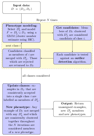
Semi-supervised learning

The idea behind semi-supervised learning is to use labelled observations to guide the determination of relevant structure in the unlabelled data. The figures below described the phenoDisco algorithm described in Breckels et al. (2013).

Semi-supervised learning and novelty detection

Deep learning in R

This book focuses on introductory material in R. This shouldn’t however give the impression that more modern approaches are not available. R has plenty of activity arounds deep learning such as, for example, the keras package, an interface to Keras, a high-level neural networks API.

See this blog for an introduction.

6.2 Model performance

When investigating multi-class problems, it is good to consider additional performance metrics and to inspect the confusion matrices in more details, to look if some classes suffer from greater mis-classification rates.

Models accuracy can also evaluated using the F1 score, where \(F1 = 2 ~ \frac{precision \times recall}{precision + recall}\), calculated as the harmonic mean of the precision (\(precision = \frac{tp}{tp+fp}\), a measure of exactness – returned output is a relevant result) and recall (\(recall=\frac{tp}{tp+fn}\), a measure of completeness – indicating how much was missed from the output). What we are aiming for are high generalisation accuracy, i.e high \(F1\), indicating that the marker proteins in the test data set are consistently and correctly assigned by the algorithms.

For a multi-class problem, the macro F1 (mean of class F1s) can be used.

6.3 Credit and acknowledgements

Many parts of this course have been influenced by the DataCamp’s Machine Learning with R skill track, in particular the Machine Learning Toolbox (supervised learning chapter) and the Unsupervised Learning in R (unsupervised learning chapter) courses.

Jamie Lendrum has addressed numerous typos in the first version.

The very hands-on approach has also been influenced by the Software and Data Carpentry lessons and teaching styles.

6.4 References and further reading

caret: Classification and Regression Training. Max Kuhn. https://CRAN.R-project.org/package=caret.
Applied predictive modeling, Max Kuhn and Kjell Johnson (book webpage http://appliedpredictivemodeling.com/) and the caret book.
An Introduction to Statistical Learning (with Applications in R). Gareth James, Daniela Witten, Trevor Hastie and Robert Tibshirani.
mlr: Machine Learning in R. Bischl B, Lang M, Kotthoff L, Schiffner J, Richter J, Studerus E, Casalicchio G and Jones Z (2016). Journal of Machine Learning Research, 17(170), pp. 1-5. https://github.com/mlr-org/mlr.
DataCamp’s Machine Learning with R skill track (requires paid access).

6.5 Session information

sessionInfo()

## R version 3.6.2 (2019-12-12)
## Platform: x86_64-pc-linux-gnu (64-bit)
## Running under: Ubuntu 18.04.4 LTS
## 
## Matrix products: default
## BLAS:   /usr/lib/x86_64-linux-gnu/atlas/libblas.so.3.10.3
## LAPACK: /usr/lib/x86_64-linux-gnu/atlas/liblapack.so.3.10.3
## 
## locale:
##  [1] LC_CTYPE=en_US.UTF-8       LC_NUMERIC=C              
##  [3] LC_TIME=fr_FR.UTF-8        LC_COLLATE=en_US.UTF-8    
##  [5] LC_MONETARY=fr_FR.UTF-8    LC_MESSAGES=en_US.UTF-8   
##  [7] LC_PAPER=fr_FR.UTF-8       LC_NAME=C                 
##  [9] LC_ADDRESS=C               LC_TELEPHONE=C            
## [11] LC_MEASUREMENT=fr_FR.UTF-8 LC_IDENTIFICATION=C       
## 
## attached base packages:
## [1] stats     graphics  grDevices utils     datasets  methods   base     
## 
## other attached packages:
##  [1] Rtsne_0.15          modeldata_0.0.1     MASS_7.3-51.5      
##  [4] kernlab_0.9-29      impute_1.60.0       randomForest_4.6-14
##  [7] rpart.plot_3.0.8    rpart_4.1-15        ranger_0.12.1      
## [10] caTools_1.18.0      class_7.3-15        knitr_1.28         
## [13] DT_0.12             naivebayes_0.9.6    glmnet_3.0-2       
## [16] Matrix_1.2-18       caret_6.0-85        lattice_0.20-40    
## [19] C50_0.1.3           mlbench_2.1-1       scales_1.1.0       
## [22] ggplot2_3.2.1       BiocStyle_2.14.4    dplyr_0.8.4        
## 
## loaded via a namespace (and not attached):
##  [1] nlme_3.1-144         bitops_1.0-6         lubridate_1.7.4     
##  [4] tools_3.6.2          R6_2.4.1             lazyeval_0.2.2      
##  [7] colorspace_1.4-1     nnet_7.3-12          withr_2.1.2         
## [10] tidyselect_1.0.0     compiler_3.6.2       Cubist_0.2.3        
## [13] bookdown_0.17        mvtnorm_1.0-12       stringr_1.4.0       
## [16] digest_0.6.24        rmarkdown_2.1        pkgconfig_2.0.3     
## [19] htmltools_0.4.0      fastmap_1.0.1        highr_0.8           
## [22] htmlwidgets_1.5.1    rlang_0.4.4          rstudioapi_0.11     
## [25] shiny_1.4.0          shape_1.4.4          generics_0.0.2      
## [28] farver_2.0.3         jsonlite_1.6.1       crosstalk_1.0.0     
## [31] ModelMetrics_1.2.2.1 magrittr_1.5         Formula_1.2-3       
## [34] Rcpp_1.0.3           munsell_0.5.0        partykit_1.2-6      
## [37] lifecycle_0.1.0      stringi_1.4.5        pROC_1.16.1         
## [40] yaml_2.2.1           inum_1.0-1           plyr_1.8.5          
## [43] recipes_0.1.9        grid_3.6.2           promises_1.1.0      
## [46] crayon_1.3.4         splines_3.6.2        pillar_1.4.3        
## [49] reshape2_1.4.3       codetools_0.2-16     stats4_3.6.2        
## [52] glue_1.3.1           evaluate_0.14        data.table_1.12.8   
## [55] BiocManager_1.30.10  httpuv_1.5.2         foreach_1.4.8       
## [58] RANN_2.6.1           gtable_0.3.0         purrr_0.3.3         
## [61] assertthat_0.2.1     xfun_0.12            gower_0.2.1         
## [64] mime_0.9             prodlim_2019.11.13   libcoin_1.0-5       
## [67] xtable_1.8-4         e1071_1.7-3          later_1.0.0         
## [70] survival_3.1-8       timeDate_3043.102    tibble_2.1.3        
## [73] iterators_1.0.12     lava_1.6.6           ipred_0.9-9

There are exactly 238 available methods. See http://topepo.github.io/caret/train-models-by-tag.html for details.↩