Chapter 5 Supervised Learning

5.1 Introduction

In supervised learning (SML), the learning algorithm is presented with labelled example inputs, where the labels indicate the desired output. SML itself is composed of classification, where the output is qualitative, and regression, where the output is quantitative.

When two sets of labels, or classes, are available, one speaks of binary classification. A classical example thereof is labelling an email as spam or not spam. When more classes are to be learnt, one speaks of a multi-class problem, such as annotation of a new Iris example as being from the setosa, versicolor or virginica species. In these cases, the output is a single label (of one of the anticipated classes). If multiple labels may be assigned to each example, one speaks of multi-label classification.

5.2 Preview

To start this chapter, let’s use a simple, but useful classification algorithm, k-nearest neighbours (kNN) to classify the iris flowers. We will use the knn function from the class package.

K-nearest neighbours works by directly measuring the (Euclidean) distance between observations and inferring the class of unlabelled data from the class of its nearest neighbours. In the figure below, the unlabelled instances 1 and 2 will be assigned classes c1 (blue) and c2 (red) as their closest neighbours are red and blue, respectively.

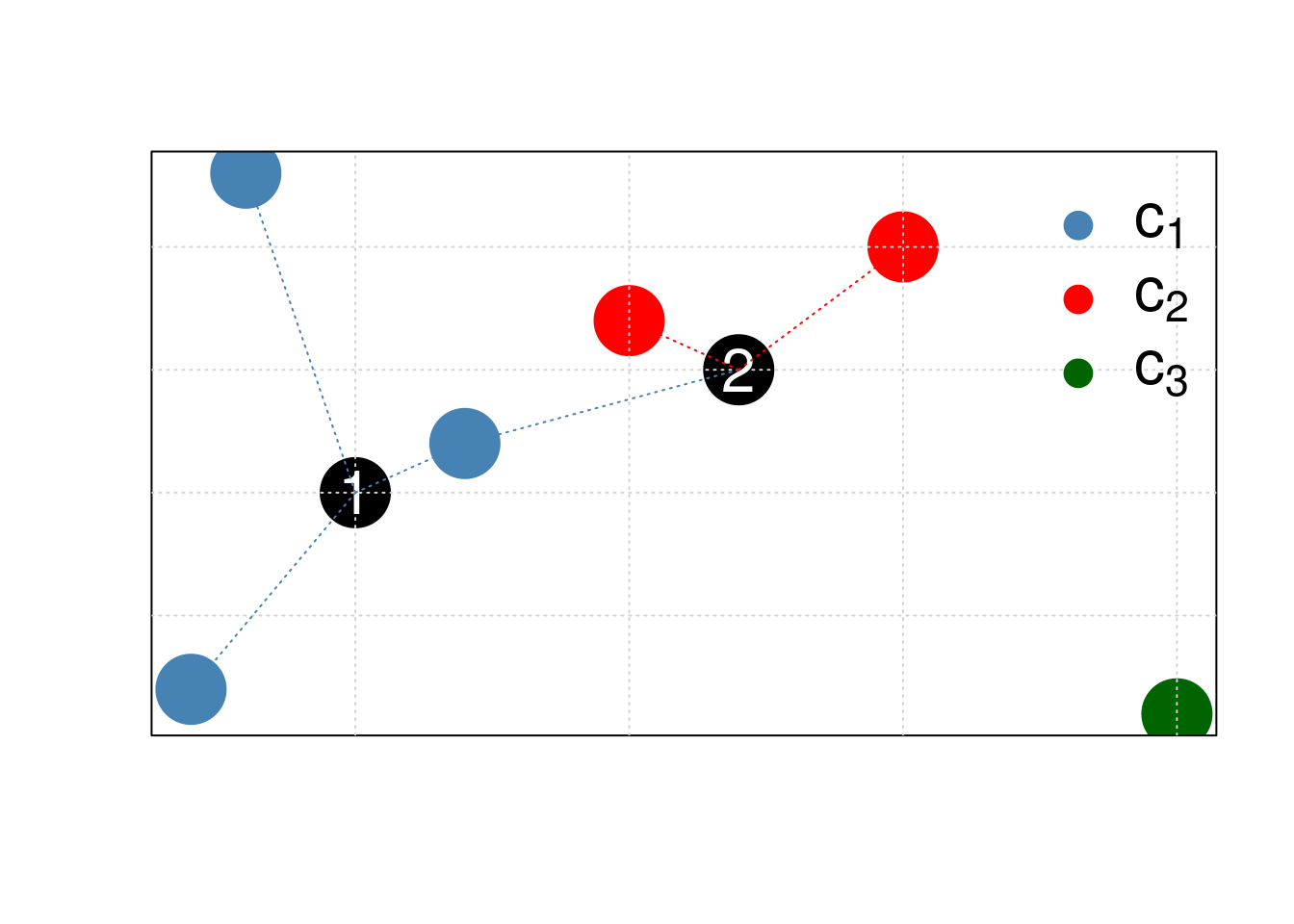
Figure 5.1: Schematic illustrating the k nearest neighbors algorithm.

Typically in machine learning, there are two clear steps, where one first trains a model and then uses the model to predict new outputs (class labels in this case). In the kNN, these two steps are combined into a single function call to knn.

Lets draw a set of 50 random iris observations to train the model and predict the species of another set of 50 randomly chosen flowers. The knn function takes the training data, the new data (to be inferred) and the labels of the training data, and returns (by default) the predicted class.

set.seed(12L)
tr <- sample(150, 50)
nw <- sample(150, 50)
library("class")
knnres <- knn(iris[tr, -5], iris[nw, -5], iris$Species[tr])
head(knnres)

## [1] versicolor setosa     versicolor setosa     setosa     setosa    
## Levels: setosa versicolor virginica

We can now compare the observed kNN-predicted class and the expected known outcome and calculate the overall accuracy of our model.

table(knnres, iris$Species[nw])

##             
## knnres       setosa versicolor virginica
##   setosa         20          0         0
##   versicolor      0         17         2
##   virginica       0          0        11

mean(knnres == iris$Species[nw])

## [1] 0.96

We have omitted an important argument from knn, which is the parameter k of the classifier. This parameter defines how many nearest neighbours will be considered to assign a class to a new unlabelled observation. From the arguments of the function,

args(knn)

## function (train, test, cl, k = 1, l = 0, prob = FALSE, use.all = TRUE) 
## NULL

we see that the default value is 1. But is this a good value? Wouldn’t we prefer to look at more neighbours and infer the new class using a vote based on more labels?

Challenge

Repeat the kNN classification above by using another value of k, and compare the accuracy of this new model to the one above. Make sure to use the same tr and nw training and new data to avoid any biases in the comparison.

knnres5 <- knn(iris[tr, -5], iris[nw, -5], iris$Species[tr], k = 5)
mean(knnres5 == iris$Species[nw])

## [1] 0.94

table(knnres5, knnres)

##             knnres
## knnres5      setosa versicolor virginica
##   setosa         20          0         0
##   versicolor      0         19         1
##   virginica       0          0        10

Challenge

Rerun the kNN classifier with a value of k > 1, and specify prob = TRUE to obtain the proportion of the votes for the winning class.

knnres5prob <- knn(iris[tr, -5], iris[nw, -5], iris$Species[tr], k = 5, prob = TRUE)
table(attr(knnres5prob, "prob"))

## 
##               0.6               0.8 0.833333333333333                 1 
##                 3                13                 1                33

This introductory example leads to two important and related questions that we need to consider:

How can we do a good job in training and testing data? In the example above, we choose random training and new data.
How can we estimate our model parameters (k in the example above) so as to obtain good classification accuracy?

5.3 Model performance

5.3.1 In-sample and out-of-sample error

In supervised machine learning, we have a desired output and thus know precisely what is to be computed. It thus becomes possible to directly evaluate a model using a quantifiable and objective metric. For regression, we will use the root mean squared error (RMSE), which is what linear regression (lm in R) seeks to minimise. For classification, we will use model prediction accuracy.

Typically, we won’t want to calculate any of these metrics using observations that were also used to calculate the model. This approach, called in-sample error leads to optimistic assessment of our model. Indeed, the model has already seen these data upon construction, and is considered optimised for these observations in particular; it is said to over-fit the data. We prefer to calculate an out-of-sample error, on new data, to gain a better idea of how to model performs on unseen data, and estimate how well the model generalises.

In this course, we will focus on the caret package for Classification And REgression Training (see also https://topepo.github.io/caret/index.html). It provides a common and consistent interface to many, often repetitive, tasks in supervised learning.

library("caret")

The code chunk below uses the lm function to model the price of round cut diamonds and then predicts the price of these very same diamonds with the predict function.

data(diamonds)
model <- lm(price ~ ., diamonds)
p <- predict(model, diamonds)

Challenge

Calculate the root mean squared error for the prediction above

## Error on prediction
error <- p - diamonds$price
rmse_in <- sqrt(mean(error^2)) ## in-sample RMSE
rmse_in

## [1] 1129.843

Let’s now repeat the exercise above, but by calculating the out-of-sample RMSE. We prepare a 80/20 split of the data and use 80% to fit our model, and predict the target variable (this is called the training data), the price, on the 20% of unseen data (the testing data).

Challenge

Let’s create a random 80/20 split to define the test and train subsets.

Train a regression model on the training data.

Test the model on the testing data.

Calculating the out-of-sample RMSE.

set.seed(42)
ntest <- nrow(diamonds) * 0.80
test <- sample(nrow(diamonds), ntest)
model <- lm(price ~ ., data = diamonds[test, ])
p <- predict(model, diamonds[-test, ])
error <- p - diamonds$price[-test]
rmse_out <- sqrt(mean(error^2)) ## out-of-sample RMSE
rmse_out

## [1] 1137.466

The values for the out-of-sample RMSE will vary depending on what exact split was used. The diamonds is a rather extensive data set, and thus even when building our model using a subset of the available data (80% above), we manage to generate a model with a low RMSE, and possibly lower than the in-sample error.

When dealing with datasets of smaller sizes, however, the presence of a single outlier in the train and test data split can substantially influence the model and the RMSE. We can’t rely on such an approach and need a more robust one where we can generate and use multiple, different train/test sets to sample a set of RMSEs, leading to a better estimate of the out-of-sample RMSE.

5.3.2 Cross-validation

Instead of doing a single training/testing split, we can systematise this process, produce multiple, different out-of-sample train/test splits, that will lead to a better estimate of the out-of-sample RMSE.

The figure below illustrates the cross validation procedure, creating 3 folds. One would typically do a 10-fold cross validation (if the size of the data permits it). We split the data into 3 random and complementary folds, so that each data point appears exactly once in each fold. This leads to a total test set size that is identical to the size of the full dataset but is composed of out-of-sample predictions.

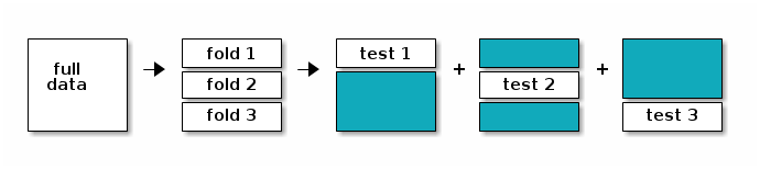
Schematic of 3-fold cross validation producing three training (blue) and testing (white) splits.

After cross-validation, all models used within each fold are discarded, and a new model is built using the whole dataset, with the best model parameter(s), i.e those that generalised over all folds.

This makes cross-validation quite time consuming, as it takes x+1 (where x in the number of cross-validation folds) times as long as fitting a single model, but is essential.

Note that it is important to maintain the class proportions within the different folds, i.e. respect the proportion of the different classes in the original data. This is also taken care when using the caret package.

The procedure of creating folds and training the models is handled by the train function in caret. Below, we apply it to the diamond price example that we used when introducing the model performance.

We start by setting a random seed to be able to reproduce the example.
We specify the method (the learning algorithm) we want to use. Here, we use "lm", but, as we will see later, there are many others to choose from¹.
We then set the out-of-sample training procedure to 10-fold cross validation (method = "cv" and number = 10). To simplify the output in the material for better readability, we set the verbosity flag to FALSE, but it is useful to set it to TRUE in interactive mode.

set.seed(42)
model <- train(price ~ ., diamonds,
               method = "lm",
               trControl = trainControl(method = "cv",
                                        number = 10,
                                        verboseIter = FALSE))
model

## Linear Regression 
## 
## 53940 samples
##     9 predictor
## 
## No pre-processing
## Resampling: Cross-Validated (10 fold) 
## Summary of sample sizes: 48547, 48545, 48546, 48545, 48546, 48546, ... 
## Resampling results:
## 
##   RMSE      Rsquared   MAE     
##   1130.819  0.9197489  740.5712
## 
## Tuning parameter 'intercept' was held constant at a value of TRUE

Once we have trained our model, we can directly use this train object as input to the predict method:

p <- predict(model, diamonds)
error <- p - diamonds$price
rmse_xval <- sqrt(mean(error^2)) ## xval RMSE
rmse_xval

## [1] 1129.843

Challenge

Train a linear model using 10-fold cross-validation and then use it to predict the median value of owner-occupied homes in Boston from the Boston dataset as described above. Then calculate the RMSE.

library("MASS")
data(Boston)
model <- train(medv ~ .,
               Boston,
               method = "lm",
               trControl = trainControl(method = "cv",
                                        number = 10))
model

## Linear Regression 
## 
## 506 samples
##  13 predictor
## 
## No pre-processing
## Resampling: Cross-Validated (10 fold) 
## Summary of sample sizes: 455, 456, 457, 456, 454, 456, ... 
## Resampling results:
## 
##   RMSE      Rsquared   MAE     
##   4.838479  0.7301286  3.433261
## 
## Tuning parameter 'intercept' was held constant at a value of TRUE

p <- predict(model, Boston)
sqrt(mean((p - Boston$medv)^2))

## [1] 4.679191

5.4 Classification performance

Above, we have used the RMSE to assess the performance of our regression model. When using a classification algorithm, we want to assess its accuracy to do so.

5.4.1 Confusion matrix

Instead of calculating an error between predicted value and known value, in classification we will directly compare the predicted class matches with the known label. To do so, rather than calculating the mean accuracy as we did above, in the introductory kNN example, we can calculate a confusion matrix.

A confusion matrix contrasts predictions to actual results. Correct results are true positives (TP) and true negatives (TN) are found along the diagonal. All other cells indicate false results, i.e false negatives (FN) and false positives (FP).

	Reference Yes	Reference No
Predicted Yes	TP	FP
Predicted No	FN	TN

The values that populate this table will depend on the cutoff that we set to define whether the classifier should predict Yes or No. Intuitively, we might want to use 0.5 as a threshold, and assign every result with a probability > 0.5 to Yes and No otherwise.

Let’s experiment with this using the Sonar dataset, and see if we can differentiate mines from rocks using a logistic classification model use the glm function from the stats package.

library("mlbench")
data(Sonar)
## 60/40 split
tr <- sample(nrow(Sonar), round(nrow(Sonar) * 0.6))
train <- Sonar[tr, ]
test <- Sonar[-tr, ]

model <- glm(Class ~ ., data = train, family = "binomial")
p <- predict(model, test, type = "response")
summary(p)

##    Min. 1st Qu.  Median    Mean 3rd Qu.    Max. 
##  0.0000  0.0000  0.8545  0.5123  1.0000  1.0000

cl <- ifelse(p > 0.5, "M", "R")
table(cl, test$Class)

##    
## cl   M  R
##   M 12 31
##   R 31  9

The caret package offers its own, more informative function to calculate a confusion matrix:

confusionMatrix(factor(cl), test$Class)

## Confusion Matrix and Statistics
## 
##           Reference
## Prediction  M  R
##          M 12 31
##          R 31  9
##                                           
##                Accuracy : 0.253           
##                  95% CI : (0.1639, 0.3604)
##     No Information Rate : 0.5181          
##     P-Value [Acc > NIR] : 1               
##                                           
##                   Kappa : -0.4959         
##                                           
##  Mcnemar's Test P-Value : 1               
##                                           
##             Sensitivity : 0.2791          
##             Specificity : 0.2250          
##          Pos Pred Value : 0.2791          
##          Neg Pred Value : 0.2250          
##              Prevalence : 0.5181          
##          Detection Rate : 0.1446          
##    Detection Prevalence : 0.5181          
##       Balanced Accuracy : 0.2520          
##                                           
##        'Positive' Class : M               
##

We get, among others

the accuracy: \(\frac{TP + TN}{TP + TN + FP + FN}\)
the sensitivity (recall, TP rate): \(\frac{TP}{TP + FN}\)
the specificity: \(\frac{TN}{TN + FP}\)
positive predictive value (precision): \(\frac{TP}{TP + FP}\)
negative predictive value: \(\frac{TN}{TN + FN}\)
FP rate (fall-out): \(\frac{FP}{FP + TN}\)

Challenge

Compare the model accuracy (or any other metric) using thresholds of 0.1 and 0.9.

confusionMatrix(factor(ifelse(p > 0.9, "M", "R")), test$Class)

## Confusion Matrix and Statistics
## 
##           Reference
## Prediction  M  R
##          M 11 30
##          R 32 10
##                                           
##                Accuracy : 0.253           
##                  95% CI : (0.1639, 0.3604)
##     No Information Rate : 0.5181          
##     P-Value [Acc > NIR] : 1.0000          
##                                           
##                   Kappa : -0.4933         
##                                           
##  Mcnemar's Test P-Value : 0.8989          
##                                           
##             Sensitivity : 0.2558          
##             Specificity : 0.2500          
##          Pos Pred Value : 0.2683          
##          Neg Pred Value : 0.2381          
##              Prevalence : 0.5181          
##          Detection Rate : 0.1325          
##    Detection Prevalence : 0.4940          
##       Balanced Accuracy : 0.2529          
##                                           
##        'Positive' Class : M               
##

confusionMatrix(factor(ifelse(p > 0.1, "M", "R")), test$Class)

## Confusion Matrix and Statistics
## 
##           Reference
## Prediction  M  R
##          M 12 31
##          R 31  9
##                                           
##                Accuracy : 0.253           
##                  95% CI : (0.1639, 0.3604)
##     No Information Rate : 0.5181          
##     P-Value [Acc > NIR] : 1               
##                                           
##                   Kappa : -0.4959         
##                                           
##  Mcnemar's Test P-Value : 1               
##                                           
##             Sensitivity : 0.2791          
##             Specificity : 0.2250          
##          Pos Pred Value : 0.2791          
##          Neg Pred Value : 0.2250          
##              Prevalence : 0.5181          
##          Detection Rate : 0.1446          
##    Detection Prevalence : 0.5181          
##       Balanced Accuracy : 0.2520          
##                                           
##        'Positive' Class : M               
##

5.4.2 Receiver operating characteristic (ROC) curve

There is no reason to use 0.5 as a threshold. One could use a low threshold to catch more mines with less certainty or or higher threshold to catch fewer mines with more certainty.

This illustrates the need to adequately balance TP and FP rates. We need to have a way to do a cost-benefit analysis, and the solution will often depend on the question/problem.

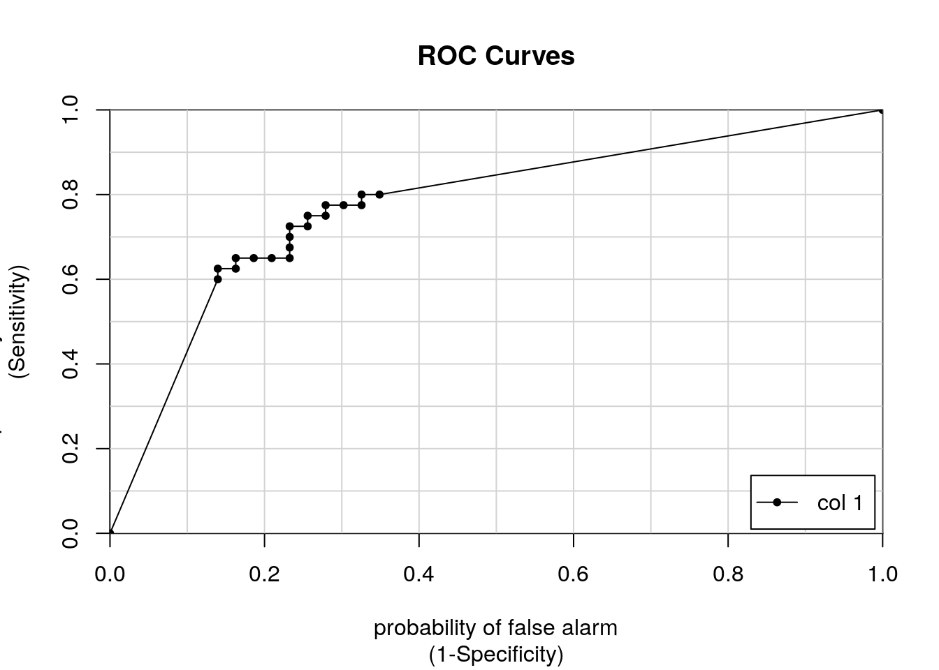
One solution would be to try with different classification thresholds. Instead of inspecting numerous confusion matrices, it is possible to automate the calculation of the TP and FP rates at each threshold and visualise all results along a ROC curve.

This can be done with the colAUC function from the caTools package:

caTools::colAUC(p, test[["Class"]], plotROC = TRUE)

##              [,1]
## M vs. R 0.7767442

x: FP rate (1 - specificity)
y: TP rate (sensitivity)
each point along the curve represents a confusion matrix for a given threshold

In addition, the colAUC function returns the area under the curve (AUC) model accuracy metric. This is single number metric, summarising the model performance along all possible thresholds:

an AUC of 0.5 corresponds to a random model
values > 0.5 do better than a random guess
a value of 1 represents a perfect model
a value 0 represents a model that is always wrong

5.4.3 AUC in `caret`

When using caret’s trainControl function to train a model, we can set it so that it computes the ROC and AUC properties for us.

## Create trainControl object: myControl
myControl <- trainControl(
    method = "cv", ## cross validation
    number = 10,   ## 10-fold
    summaryFunction = twoClassSummary, ## NEW
    classProbs = TRUE, # IMPORTANT
    verboseIter = FALSE
)
## Train glm with custom trainControl: model
model <- train(Class ~ ., Sonar,
               method = "glm", ## to use glm's logistic regression
               trControl = myControl)

## Print model to console
print(model)

## Generalized Linear Model 
## 
## 208 samples
##  60 predictor
##   2 classes: 'M', 'R' 
## 
## No pre-processing
## Resampling: Cross-Validated (10 fold) 
## Summary of sample sizes: 187, 188, 188, 187, 188, 187, ... 
## Resampling results:
## 
##   ROC       Sens       Spec     
##   0.733447  0.7477273  0.6688889

Challenge

Define a train object that uses the AUC and 10-fold cross validation to classify the Sonar data using a logistic regression, as demonstrated above.

5.5 Random forest

Random forest models are accurate and non-linear models and robust to over-fitting and hence quite popular. They however require hyperparameters to be tuned manually, like the value k in the example above.

Building a random forest starts by generating a high number of individual decision trees. A single decision tree isn’t very accurate, but many different trees built using different inputs (with bootstrapped inputs, features and observations) enable us to explore a broad search space and, once combined, produce accurate models, a technique called bootstrap aggregation or bagging.

5.5.1 Decision trees

A great advantage of decision trees is that they make a complex decision simpler by breaking it down into smaller, simpler decisions using a divide-and-conquer strategy. They basically identify a set of if-else conditions that split the data according to the value of the features.

library("rpart") ## recursive partitioning
m <- rpart(Class ~ ., data = Sonar,
           method = "class")
library("rpart.plot")
rpart.plot(m)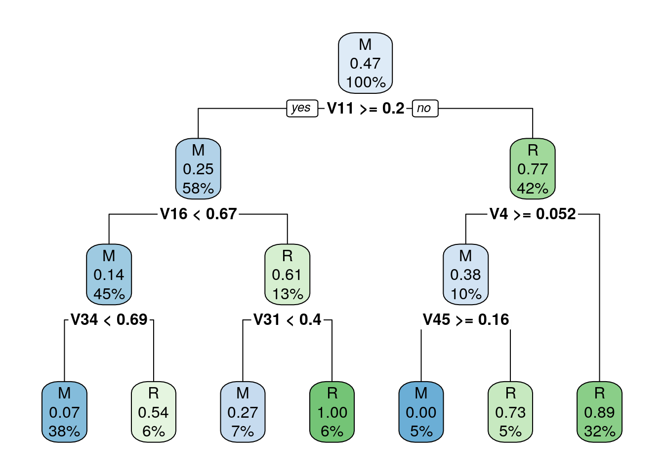

Figure 5.2: Descision tree with its if-else conditions

p <- predict(m, Sonar, type = "class")
table(p, Sonar$Class)

##    
## p    M  R
##   M 95 10
##   R 16 87

Decision trees choose splits based on most homogeneous partitions, and lead to smaller and more homogeneous partitions over their iterations.

An issue with single decision trees is that they can grow, and become large and complex with many branches, which corresponds to over-fitting. Over-fitting models noise, rather than general patterns in the data, focusing on subtle patterns (outliers) that won’t generalise.

To avoid over-fitting, individual decision trees are pruned. Pruning can happen as a pre-condition when growing the tree, or afterwards, by pruning a large tree.

Pre-pruning: stop growing process, i.e stops divide-and-conquer after a certain number of iterations (grows tree to a certain predefined level), or requires a minimum number of observations in each mode to allow splitting.
Post-pruning: grow a large and complex tree, and reduce its size; nodes and branches that have a negligible effect on the classification accuracy are removed.

5.5.2 Training a random forest

Let’s return to random forests and train a model using the train function from caret:

set.seed(12)
model <- train(Class ~ .,
               data = Sonar,
               method = "ranger")
print(model)

## Random Forest 
## 
## 208 samples
##  60 predictor
##   2 classes: 'M', 'R' 
## 
## No pre-processing
## Resampling: Bootstrapped (25 reps) 
## Summary of sample sizes: 208, 208, 208, 208, 208, 208, ... 
## Resampling results across tuning parameters:
## 
##   mtry  splitrule   Accuracy   Kappa    
##    2    gini        0.8090731  0.6131571
##    2    extratrees  0.8136902  0.6234492
##   31    gini        0.7736954  0.5423516
##   31    extratrees  0.8285153  0.6521921
##   60    gini        0.7597299  0.5140905
##   60    extratrees  0.8157646  0.6255929
## 
## Tuning parameter 'min.node.size' was held constant at a value of 1
## Accuracy was used to select the optimal model using the largest value.
## The final values used for the model were mtry = 31, splitrule = extratrees
##  and min.node.size = 1.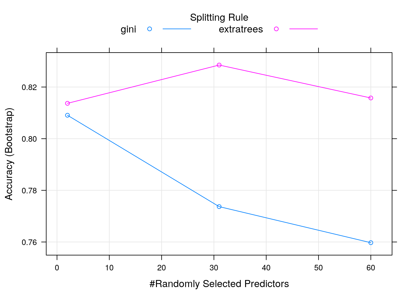

plot(model)

The main hyperparameter is mtry, i.e. the number of randomly selected variables used at each split. Two variables produce random models, while hundreds of variables tend to be less random, but risk over-fitting. The caret package can automate the tuning of the hyperparameter using a grid search, which can be parametrised by setting tuneLength (that sets the number of hyperparameter values to test) or directly defining the tuneGrid (the hyperparameter values), which requires knowledge of the model.

model <- train(Class ~ .,
               data = Sonar,
               method = "ranger",
               tuneLength = 5)

set.seed(42)
myGrid <- expand.grid(mtry = c(5, 10, 20, 40, 60),
                      splitrule = c("gini", "extratrees"),
                      min.node.size = 1) ## Minimal node size; default 1 for classification
model <- train(Class ~ .,
               data = Sonar,
               method = "ranger",
               tuneGrid = myGrid,
               trControl = trainControl(method = "cv",
                                       number = 5,
                                       verboseIter = FALSE))
print(model)

## Random Forest 
## 
## 208 samples
##  60 predictor
##   2 classes: 'M', 'R' 
## 
## No pre-processing
## Resampling: Cross-Validated (5 fold) 
## Summary of sample sizes: 166, 167, 167, 167, 165 
## Resampling results across tuning parameters:
## 
##   mtry  splitrule   Accuracy   Kappa    
##    5    gini        0.8076277  0.6098253
##    5    extratrees  0.8416579  0.6784745
##   10    gini        0.7927667  0.5799348
##   10    extratrees  0.8418848  0.6791453
##   20    gini        0.7882316  0.5718852
##   20    extratrees  0.8516355  0.6991879
##   40    gini        0.7880048  0.5716461
##   40    extratrees  0.8371229  0.6695638
##   60    gini        0.7833482  0.5613525
##   60    extratrees  0.8322448  0.6599318
## 
## Tuning parameter 'min.node.size' was held constant at a value of 1
## Accuracy was used to select the optimal model using the largest value.
## The final values used for the model were mtry = 20, splitrule = extratrees
##  and min.node.size = 1.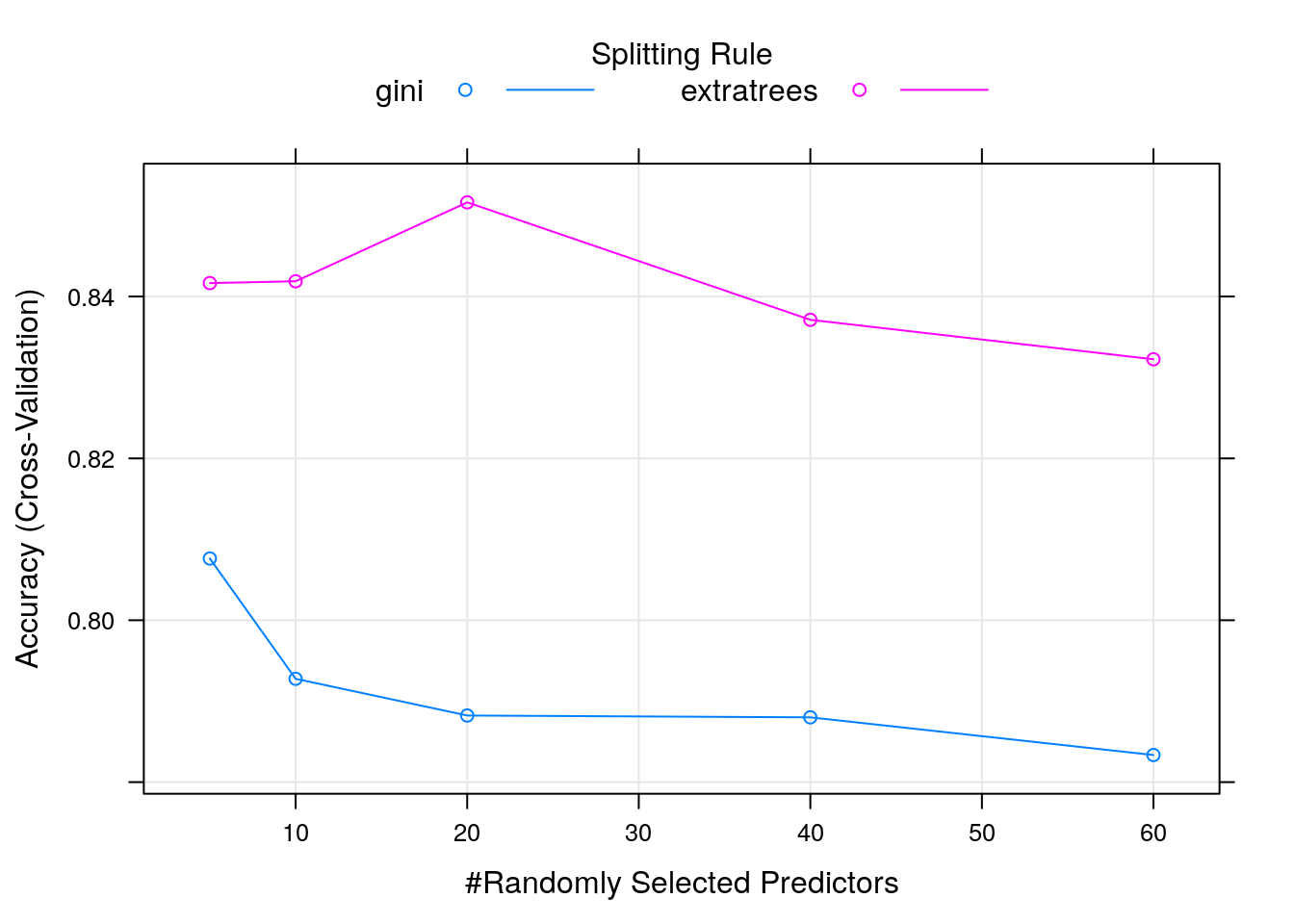

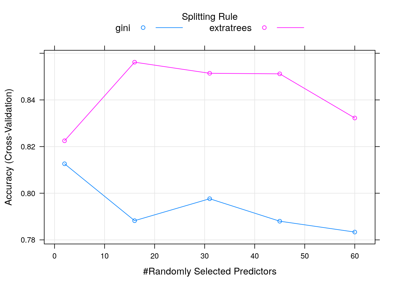
plot(model)

Challenge

Experiment with training a random forest model as described above, by using 5-fold cross validation, and setting a tuneLength of 5.

set.seed(42)
model <- train(Class ~ .,
               data = Sonar,
               method = "ranger",
               tuneLength = 5,
               trControl = trainControl(method = "cv",
                                        number = 5,
                                        verboseIter = FALSE))
plot(model)

5.6 Data pre-processing

5.6.1 Missing values

Real datasets often come with missing values. In R, these should be encoded using NA. There are basically two approaches to deal with such cases.

Drop the observations with missing values, or, if one feature contains a very high proportion of NAs, drop the feature altogether. These approaches are only applicable when the proportion of missing values is relatively small. Otherwise, it could lead to losing too much data.
Impute (replace) missing values.

Data imputation can however have critical consequences depending on the proportion of missing values and their nature. From a statistical point of view, missing values are classified as missing completely at random (MCAR), missing at random (MAR) or missing not at random (MNAR), and the type of the missing values will influence the efficiency of the imputation method.

The figure below shows how different imputation methods perform depending on the proportion and nature of missing values (from Lazar et al., on quantitative proteomics data).

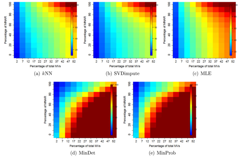
Normalised RMSE (RMSE-observation standard deviation ration) describing the effect of different imputation methods depending on the nature and proportion of the missing values: kNN (a), SVDimpute (b), MLE (c), MinDet (d), and MinProb (e).

Let’s start by simulating a dataset containing missing values using the mtcars dataset. Below, we will want to predict the mpg variable using cyl, disp, and hp, with the latter containing 10 missing values.

data(mtcars)
mtcars[sample(nrow(mtcars), 10), "hp"] <- NA
Y <- mtcars$mpg    ## target variable
X <- mtcars[, 2:4] ## predictors

If we now wanted to train a model (using the non-formula interface):

try(train(X, Y))

## note: only 2 unique complexity parameters in default grid. Truncating the grid to 2 .
## 
## Something is wrong; all the RMSE metric values are missing:
##       RMSE        Rsquared        MAE     
##  Min.   : NA   Min.   : NA   Min.   : NA  
##  1st Qu.: NA   1st Qu.: NA   1st Qu.: NA  
##  Median : NA   Median : NA   Median : NA  
##  Mean   :NaN   Mean   :NaN   Mean   :NaN  
##  3rd Qu.: NA   3rd Qu.: NA   3rd Qu.: NA  
##  Max.   : NA   Max.   : NA   Max.   : NA  
##  NA's   :2     NA's   :2     NA's   :2    
## Error : Stopping

(Note that the occurrence of the error will depend on the model chosen.)

We could perform imputation manually, but caret provides a whole range of pre-processing methods, including imputation methods, that can directly be passed when training the model.

5.6.2 Median imputation

Imputation using median of features. This method works well if the data are missing at random.

train(X, Y, preProcess = "medianImpute")

## note: only 2 unique complexity parameters in default grid. Truncating the grid to 2 .

## Random Forest 
## 
## 32 samples
##  3 predictor
## 
## Pre-processing: median imputation (3) 
## Resampling: Bootstrapped (25 reps) 
## Summary of sample sizes: 32, 32, 32, 32, 32, 32, ... 
## Resampling results across tuning parameters:
## 
##   mtry  RMSE      Rsquared   MAE     
##   2     2.345716  0.8457441  1.923509
##   3     2.433508  0.8337201  2.007780
## 
## RMSE was used to select the optimal model using the smallest value.
## The final value used for the model was mtry = 2.

Imputing using caret also allows us to optimise the imputation based on the cross validation splits, as train will do median imputation inside each fold.

5.6.3 kNN imputation

If there is a systematic bias in the missing values, then median imputation is known to produce incorrect results. kNN imputation will impute missing values using other, similar non-missing rows. The default value is 5.

train(X, Y, preProcess = "knnImpute")

## note: only 2 unique complexity parameters in default grid. Truncating the grid to 2 .

## Random Forest 
## 
## 32 samples
##  3 predictor
## 
## Pre-processing: nearest neighbor imputation (3), centered (3), scaled (3) 
## Resampling: Bootstrapped (25 reps) 
## Summary of sample sizes: 32, 32, 32, 32, 32, 32, ... 
## Resampling results across tuning parameters:
## 
##   mtry  RMSE      Rsquared   MAE     
##   2     2.603630  0.8300018  2.145504
##   3     2.635956  0.8228652  2.171091
## 
## RMSE was used to select the optimal model using the smallest value.
## The final value used for the model was mtry = 2.

5.7 Scaling and centering

We have seen in the Unsupervised learning chapter how data at different scales can substantially disrupt a learning algorithm. Scaling (division by the standard deviation) and centering (subtraction of the mean) can also be applied directly during model training by setting. Note that they are set to be applied by default prior to training.

train(X, Y, preProcess = "scale")
train(X, Y, preProcess = "center")

As we have discussed in the section on Principal Component Analysis, PCA can be used as pre-processing method, generating a set of high-variance and perpendicular predictors, preventing collinearity.

train(X, Y, preProcess = "pca")

5.7.1 Multiple pre-processing methods

It is possible to chain multiple processing methods: imputation, center, scale, pca.

train(X, Y, preProcess = c("knnImpute", "center", "scale", "pca"))

## note: only 2 unique complexity parameters in default grid. Truncating the grid to 2 .

## Random Forest 
## 
## 32 samples
##  3 predictor
## 
## Pre-processing: nearest neighbor imputation (3), centered (3), scaled
##  (3), principal component signal extraction (3) 
## Resampling: Bootstrapped (25 reps) 
## Summary of sample sizes: 32, 32, 32, 32, 32, 32, ... 
## Resampling results across tuning parameters:
## 
##   mtry  RMSE      Rsquared   MAE     
##   2     2.549263  0.8245732  2.125463
##   3     2.553001  0.8256242  2.131125
## 
## RMSE was used to select the optimal model using the smallest value.
## The final value used for the model was mtry = 2.

The pre-processing methods above represent a classical order of operations, starting with data imputation to remove missing values, then centering and scaling, prior to PCA.

For further details, see ?preProcess.

5.8 Model selection

In this final section, we are going to compare different predictive models and choose the best one using the tools presented in the previous sections.

To to so, we are going to first create a set of common training controller object with the same train/test folds and model evaluation metrics that we will re-use. This is important to guarantee fair comparison between the different models.

For this section, we are going to use the churn data. Below, we see that about 15% of the customers churn. It is important to maintain this proportion in all of the folds.

library("C50")
data(churn)

## Warning in data(churn): data set 'churn' not found

table(churnTrain$churn)/nrow(churnTrain)

## 
##       yes        no 
## 0.1449145 0.8550855

Previously, when creating a train control object, we specified the method as "cv" and the number of folds. Now, as we want the same folds to be re-used over multiple model training rounds, we are going to pass the train/test splits directly. These splits are created with the createFolds function, which creates a list (here of length 5) containing the element indices for each fold.

myFolds <- createFolds(churnTrain$churn, k = 5)
str(myFolds)

## List of 5
##  $ Fold1: int [1:667] 3 7 13 17 20 36 39 48 52 62 ...
##  $ Fold2: int [1:667] 4 10 12 24 25 29 41 42 47 50 ...
##  $ Fold3: int [1:667] 6 15 19 21 22 26 28 32 33 34 ...
##  $ Fold4: int [1:666] 5 9 16 30 31 37 44 45 46 53 ...
##  $ Fold5: int [1:666] 1 2 8 11 14 18 23 27 35 43 ...

Challenge

Verify that the folds maintain the proportion of yes/no results.

sapply(myFolds, function(i) {
    table(churnTrain$churn[i])/length(i)
})

##         Fold1     Fold2     Fold3     Fold4     Fold5
## yes 0.1454273 0.1454273 0.1454273 0.1441441 0.1441441
## no  0.8545727 0.8545727 0.8545727 0.8558559 0.8558559

We can now a train control object to be reused consistently for different model trainings.

myControl <- trainControl(
  summaryFunction = twoClassSummary,
  classProb = TRUE,
  verboseIter = FALSE,
  savePredictions = TRUE,
  index = myFolds
)

5.8.1 `glmnet` model

The glmnet is a linear model with built-in variable selection and coefficient regularisation.

glm_model <- train(churn ~ .,
                   churnTrain,
                   metric = "ROC",
                   method = "glmnet",
                   tuneGrid = expand.grid(
                       alpha = 0:1,
                       lambda = 0:10/10),
                   trControl = myControl)
print(glm_model)

## glmnet 
## 
## 3333 samples
##   19 predictor
##    2 classes: 'yes', 'no' 
## 
## No pre-processing
## Resampling: Bootstrapped (5 reps) 
## Summary of sample sizes: 667, 667, 667, 666, 666 
## Resampling results across tuning parameters:
## 
##   alpha  lambda  ROC        Sens         Spec     
##   0      0.0     0.7575175  0.249475840  0.9567544
##   0      0.1     0.7769689  0.070920191  0.9921053
##   0      0.2     0.7785410  0.016561567  0.9986842
##   0      0.3     0.7784171  0.004659196  0.9994737
##   0      0.4     0.7780007  0.000000000  1.0000000
##   0      0.5     0.7775646  0.000000000  1.0000000
##   0      0.6     0.7771289  0.000000000  1.0000000
##   0      0.7     0.7767893  0.000000000  1.0000000
##   0      0.8     0.7764375  0.000000000  1.0000000
##   0      0.9     0.7761664  0.000000000  1.0000000
##   0      1.0     0.7759360  0.000000000  1.0000000
##   1      0.0     0.7200047  0.291397893  0.9434211
##   1      0.1     0.5216114  0.000000000  1.0000000
##   1      0.2     0.5000000  0.000000000  1.0000000
##   1      0.3     0.5000000  0.000000000  1.0000000
##   1      0.4     0.5000000  0.000000000  1.0000000
##   1      0.5     0.5000000  0.000000000  1.0000000
##   1      0.6     0.5000000  0.000000000  1.0000000
##   1      0.7     0.5000000  0.000000000  1.0000000
##   1      0.8     0.5000000  0.000000000  1.0000000
##   1      0.9     0.5000000  0.000000000  1.0000000
##   1      1.0     0.5000000  0.000000000  1.0000000
## 
## ROC was used to select the optimal model using the largest value.
## The final values used for the model were alpha = 0 and lambda = 0.2.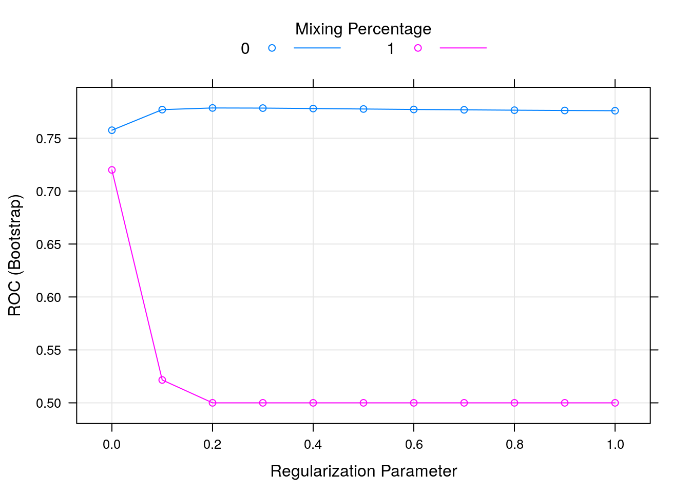

plot(glm_model)

Below, we are going to repeat this same modelling with a variety of different classifiers, some of which we haven’t looked at. This illustrates another advantage of of using meta-packages such as caret, that provide a consistant interface to different backends (in this case for machine learning). Once we have mastered the interface, it becomes easy to apply it to a new backend.

Note that some of the model training below will take some time to run, depending on the tuning parameter settings.

5.8.2 random forest model

Challenge

Apply a random forest model, making sure you reuse the same train control object.

rf_model <- train(churn ~ .,
                  churnTrain,
                  metric = "ROC",
                  method = "ranger",
                  tuneGrid = expand.grid(
                      mtry = c(2, 5, 10, 19),
                      splitrule = c("gini", "extratrees"),
                      min.node.size = 1),
                  trControl = myControl)
print(rf_model)

## Random Forest 
## 
## 3333 samples
##   19 predictor
##    2 classes: 'yes', 'no' 
## 
## No pre-processing
## Resampling: Bootstrapped (5 reps) 
## Summary of sample sizes: 667, 667, 667, 666, 666 
## Resampling results across tuning parameters:
## 
##   mtry  splitrule   ROC        Sens        Spec     
##    2    gini        0.8652359  0.02331205  0.9999123
##    2    extratrees  0.8297199  0.00000000  1.0000000
##    5    gini        0.8876968  0.20913497  0.9974561
##    5    extratrees  0.8729902  0.04659731  0.9995614
##   10    gini        0.8936162  0.39389083  0.9923684
##   10    extratrees  0.8872372  0.20134956  0.9974561
##   19    gini        0.8977501  0.58076073  0.9850000
##   19    extratrees  0.8956725  0.35972205  0.9914035
## 
## Tuning parameter 'min.node.size' was held constant at a value of 1
## ROC was used to select the optimal model using the largest value.
## The final values used for the model were mtry = 19, splitrule = gini
##  and min.node.size = 1.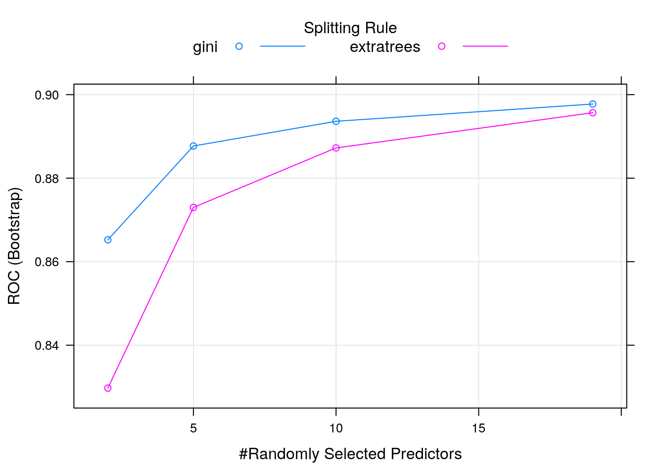

plot(rf_model)

5.8.3 kNN model

Challenge

Apply a kNN model, making sure you reuse the same train control object.

knn_model <- train(churn ~ .,
                   churnTrain,
                   metric = "ROC",
                   method = "knn",
                   tuneLength = 20,
                   trControl = myControl)
print(knn_model)

## k-Nearest Neighbors 
## 
## 3333 samples
##   19 predictor
##    2 classes: 'yes', 'no' 
## 
## No pre-processing
## Resampling: Bootstrapped (5 reps) 
## Summary of sample sizes: 667, 667, 667, 666, 666 
## Resampling results across tuning parameters:
## 
##   k   ROC        Sens        Spec     
##    5  0.6598643  0.21377542  0.9773684
##    7  0.6686225  0.19773199  0.9846491
##    9  0.6769357  0.18012612  0.9898246
##   11  0.6821201  0.16097388  0.9910526
##   13  0.6902054  0.15114003  0.9924561
##   15  0.6910103  0.14441231  0.9941228
##   17  0.6935052  0.13199047  0.9945614
##   19  0.6944057  0.12422782  0.9951754
##   21  0.6956445  0.11853369  0.9957018
##   23  0.6970316  0.10767027  0.9968421
##   25  0.6990557  0.10249562  0.9969298
##   27  0.6990448  0.09835054  0.9975439
##   29  0.7013191  0.08385883  0.9979825
##   31  0.7011835  0.07816471  0.9981579
##   33  0.7023618  0.06988258  0.9984211
##   35  0.7026399  0.06160314  0.9985965
##   37  0.7041429  0.05487408  0.9985088
##   39  0.7034029  0.04918397  0.9988596
##   41  0.7027796  0.04452745  0.9991228
##   43  0.7026078  0.03883199  0.9992105
## 
## ROC was used to select the optimal model using the largest value.
## The final value used for the model was k = 37.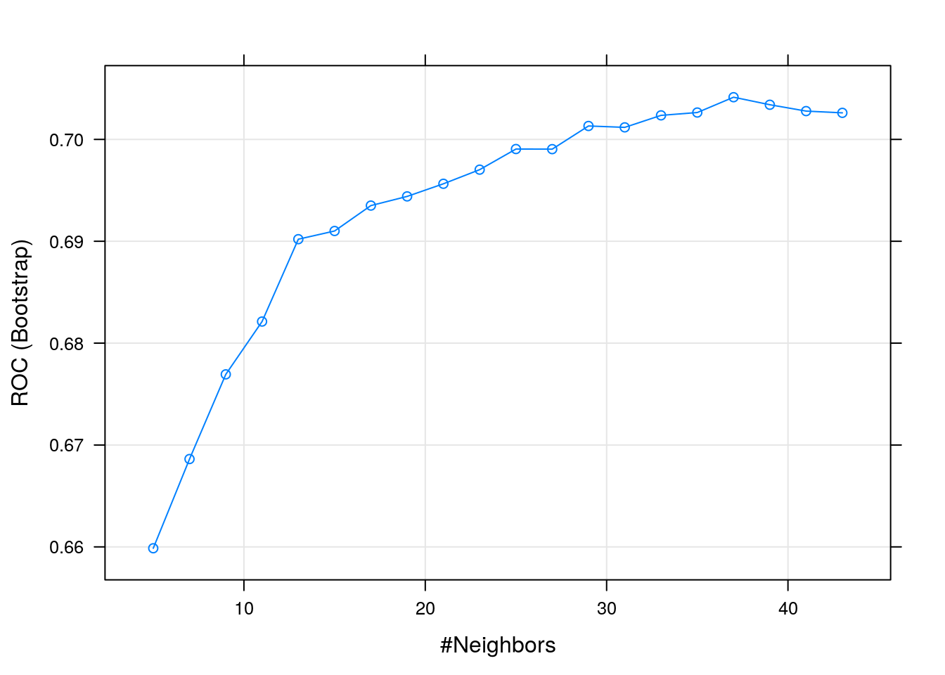

plot(knn_model)

5.8.4 Support vector machine model

Challenge

Apply a svm model, making sure you reuse the same train control object. Hint: Look at names(getModelInfo()) for all possible model names.

svm_model <- train(churn ~ .,
                   churnTrain,
                   metric = "ROC",
                   method = "svmRadial",
                   tuneLength = 10,
                   trControl = myControl)
print(svm_model)

## Support Vector Machines with Radial Basis Function Kernel 
## 
## 3333 samples
##   19 predictor
##    2 classes: 'yes', 'no' 
## 
## No pre-processing
## Resampling: Bootstrapped (5 reps) 
## Summary of sample sizes: 667, 667, 667, 666, 666 
## Resampling results across tuning parameters:
## 
##   C       ROC        Sens        Spec     
##     0.25  0.8079660  0.07454446  0.9907895
##     0.50  0.8078943  0.06003936  0.9943860
##     1.00  0.8079884  0.09215836  0.9890351
##     2.00  0.8081908  0.13717315  0.9813158
##     4.00  0.8131150  0.13920419  0.9859649
##     8.00  0.8156179  0.12888300  0.9879825
##    16.00  0.8096085  0.17804689  0.9821930
##    32.00  0.8032513  0.15837383  0.9836842
##    64.00  0.7985012  0.17082112  0.9810526
##   128.00  0.7965813  0.15939002  0.9826316
## 
## Tuning parameter 'sigma' was held constant at a value of 0.007417943
## ROC was used to select the optimal model using the largest value.
## The final values used for the model were sigma = 0.007417943 and C = 8.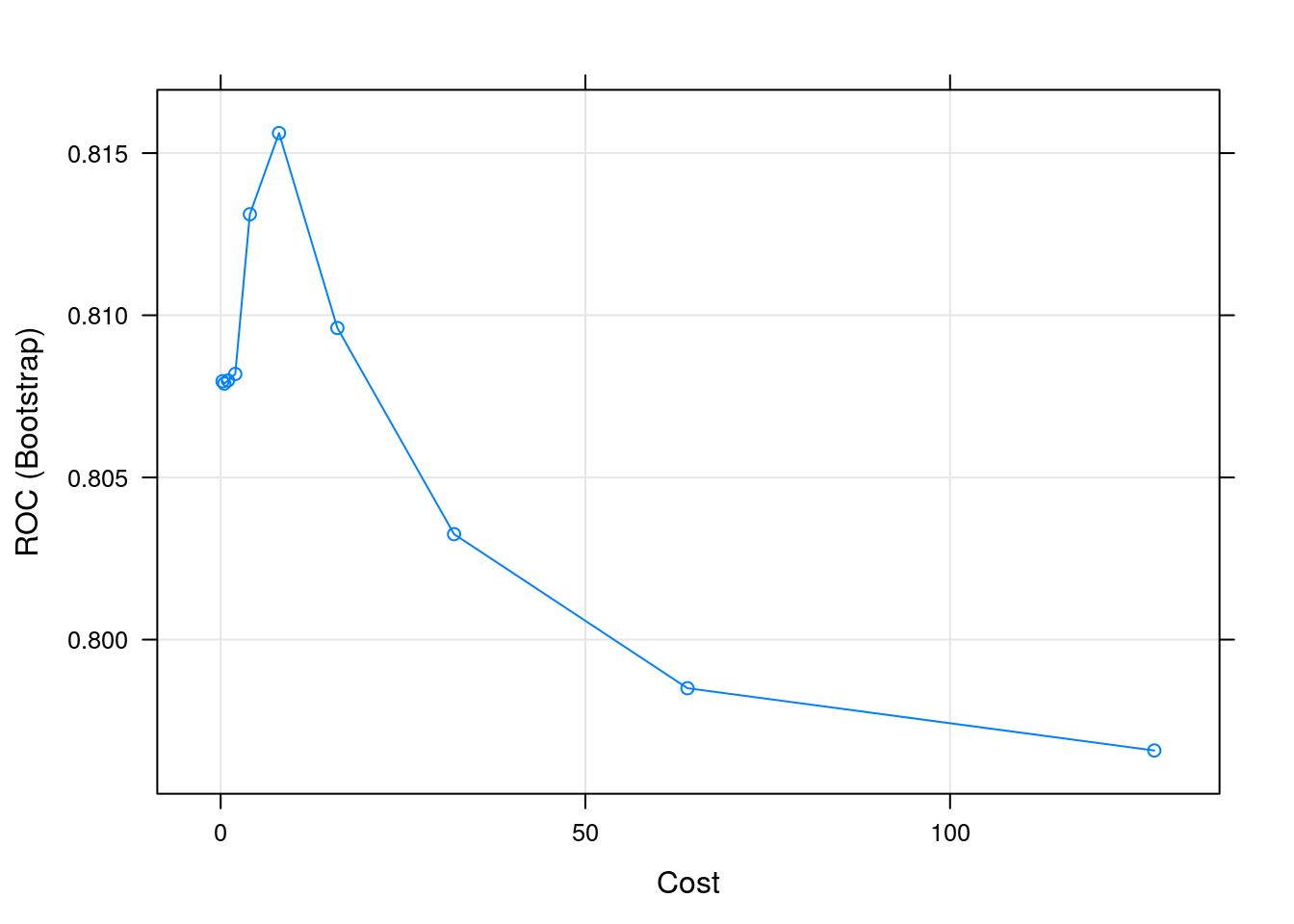

plot(svm_model)

5.8.5 Naive Bayes

Challenge

Apply a naive Bayes model, making sure you reuse the same train control object.

nb_model <- train(churn ~ .,
                  churnTrain,
                  metric = "ROC",
                  method = "naive_bayes",
                  trControl = myControl)

print(nb_model)

## Naive Bayes 
## 
## 3333 samples
##   19 predictor
##    2 classes: 'yes', 'no' 
## 
## No pre-processing
## Resampling: Bootstrapped (5 reps) 
## Summary of sample sizes: 667, 667, 667, 666, 666 
## Resampling results across tuning parameters:
## 
##   usekernel  ROC        Sens       Spec      
##   FALSE      0.5540359  0.9497409  0.07912281
##    TRUE      0.8086525  0.0000000  1.00000000
## 
## Tuning parameter 'laplace' was held constant at a value of 0
## Tuning
##  parameter 'adjust' was held constant at a value of 1
## ROC was used to select the optimal model using the largest value.
## The final values used for the model were laplace = 0, usekernel = TRUE
##  and adjust = 1.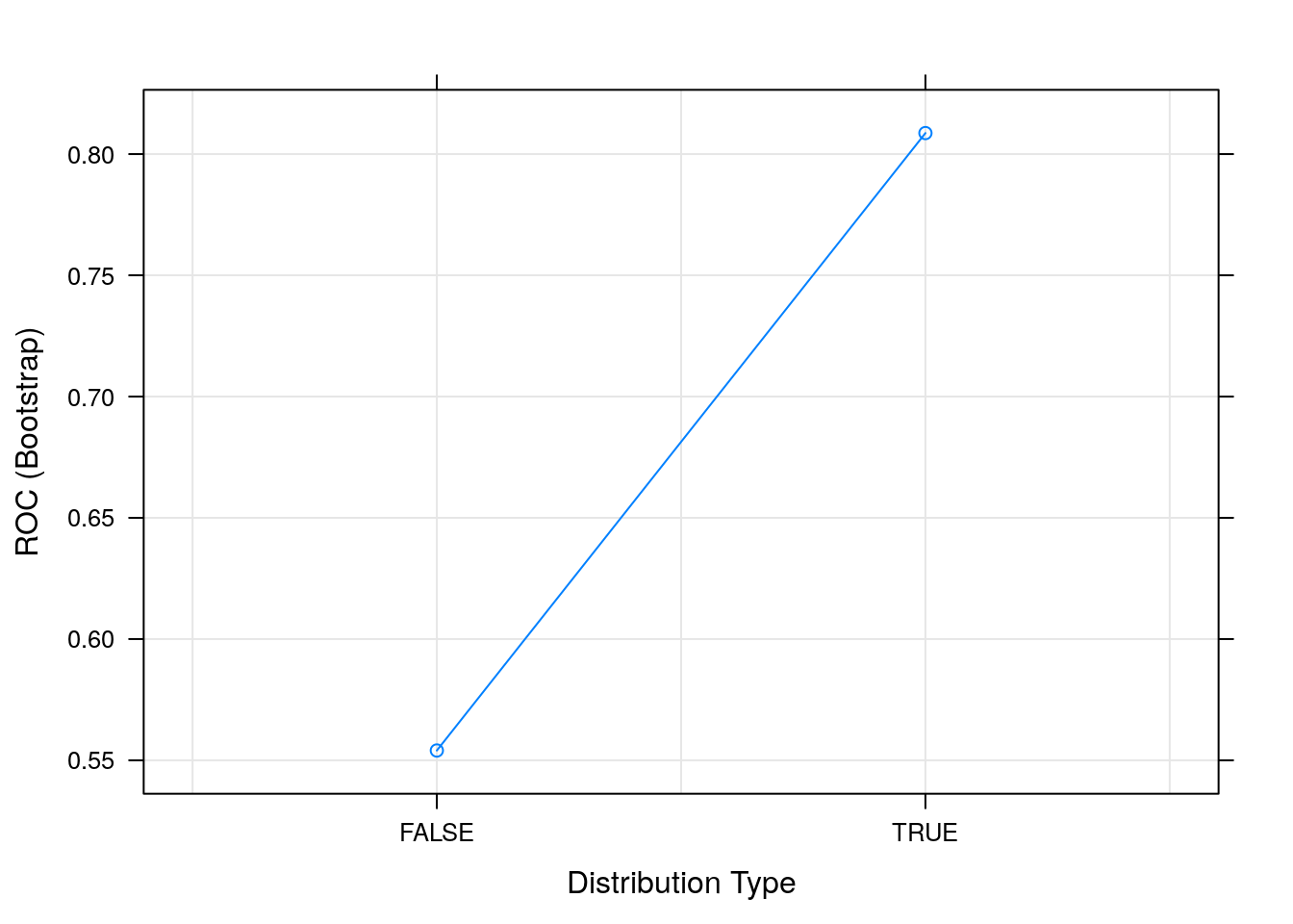

plot(nb_model)

5.8.6 Comparing models

We can now use the caret::resamples function that will compare the models and pick the one with the highest AUC and lowest AUC standard deviation.

model_list <- list(glmmet = glm_model,
                   rf = rf_model,
                   knn = knn_model,
                   svm = svm_model,
                   nb = nb_model)
resamp <- resamples(model_list)
resamp

## 
## Call:
## resamples.default(x = model_list)
## 
## Models: glmmet, rf, knn, svm, nb 
## Number of resamples: 5 
## Performance metrics: ROC, Sens, Spec 
## Time estimates for: everything, final model fit

summary(resamp)

## 
## Call:
## summary.resamples(object = resamp)
## 
## Models: glmmet, rf, knn, svm, nb 
## Number of resamples: 5 
## 
## ROC 
##             Min.   1st Qu.    Median      Mean   3rd Qu.      Max. NA's
## glmmet 0.7739183 0.7755329 0.7801770 0.7785410 0.7813153 0.7817614    0
## rf     0.8834362 0.8924689 0.8982229 0.8977501 0.9050575 0.9095653    0
## knn    0.6895458 0.7018430 0.7074902 0.7041429 0.7091369 0.7126983    0
## svm    0.8041321 0.8094912 0.8188858 0.8156179 0.8220173 0.8235629    0
## nb     0.7954270 0.8004363 0.8118887 0.8086525 0.8157215 0.8197891    0
## 
## Sens 
##               Min.    1st Qu.     Median       Mean    3rd Qu.       Max. NA's
## glmmet 0.007772021 0.01291990 0.01813472 0.01656157 0.02072539 0.02325581    0
## rf     0.511627907 0.54663212 0.58808290 0.58076073 0.62015504 0.63730570    0
## knn    0.012919897 0.02590674 0.06476684 0.05487408 0.08010336 0.09067358    0
## svm    0.106217617 0.11111111 0.12953368 0.12888300 0.14470284 0.15284974    0
## nb     0.000000000 0.00000000 0.00000000 0.00000000 0.00000000 0.00000000    0
## 
## Spec 
##             Min.   1st Qu.    Median      Mean   3rd Qu.      Max. NA's
## glmmet 0.9973684 0.9982456 0.9986842 0.9986842 0.9991228 1.0000000    0
## rf     0.9763158 0.9820175 0.9846491 0.9850000 0.9907895 0.9912281    0
## knn    0.9969298 0.9978070 0.9982456 0.9985088 0.9995614 1.0000000    0
## svm    0.9828947 0.9881579 0.9885965 0.9879825 0.9890351 0.9912281    0
## nb     1.0000000 1.0000000 1.0000000 1.0000000 1.0000000 1.0000000    0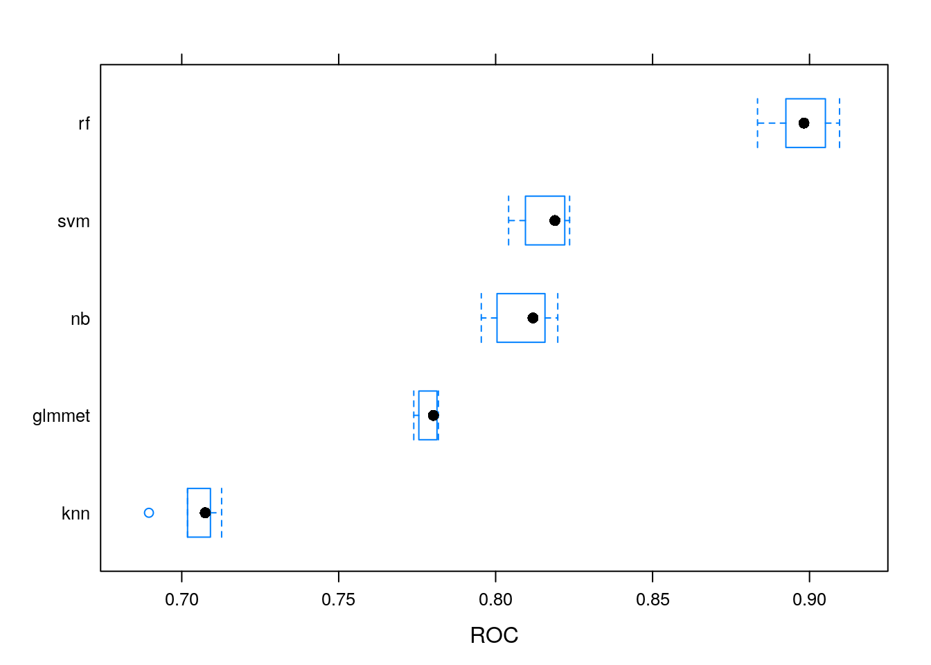

lattice::bwplot(resamp, metric = "ROC")

Figure 5.3: Comparing distributions of AUC values for various models.

5.8.7 Pre-processing

The random forest appears to be the best one. This might be related to its ability to cope well with different types of input and require little pre-processing.

Challenge

If you haven’t done so, consider pre-processing the data prior to training for a model that didn’t perform well and assess whether pre-processing affected the modelling.

svm_model1 <- train(churn ~ .,
                    churnTrain,
                    metric = "ROC",
                    method = "svmRadial",
                    tuneLength = 10,
                    trControl = myControl)

svm_model2 <- train(churn ~ .,
                    churnTrain[, c(2, 6:20)],
                    metric = "ROC",
                    method = "svmRadial",
                    preProcess = c("scale", "center", "pca"),
                    tuneLength = 10,
                    trControl = myControl)

model_list <- list(svm1 = svm_model1,
                   svm2 = svm_model2)
resamp <- resamples(model_list)
summary(resamp)

## 
## Call:
## summary.resamples(object = resamp)
## 
## Models: svm1, svm2 
## Number of resamples: 5 
## 
## ROC 
##           Min.   1st Qu.    Median      Mean   3rd Qu.      Max. NA's
## svm1 0.8036629 0.8092821 0.8188131 0.8153931 0.8215560 0.8236513    0
## svm2 0.8114933 0.8203550 0.8211070 0.8233570 0.8297328 0.8340969    0
## 
## Sens 
##           Min.   1st Qu.    Median      Mean   3rd Qu.      Max. NA's
## svm1 0.1062176 0.1295337 0.1472868 0.1614746 0.2067183 0.2176166    0
## svm2 0.3875969 0.3963731 0.4196891 0.4120148 0.4237726 0.4326425    0
## 
## Spec 
##           Min.   1st Qu.    Median      Mean   3rd Qu.      Max. NA's
## svm1 0.9745614 0.9828947 0.9842105 0.9847368 0.9890351 0.9929825    0
## svm2 0.9736842 0.9745614 0.9745614 0.9769298 0.9780702 0.9837719    0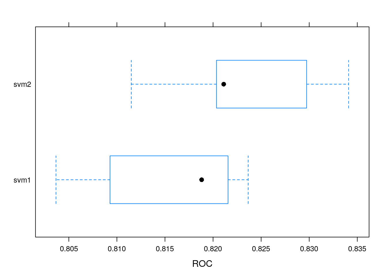

bwplot(resamp, metric = "ROC")

5.8.8 Predict using the best model

Challenge

Choose the best model using the resamples function and comparing the results and apply it to predict the churnTest labels.

p <- predict(rf_model, churnTest)
confusionMatrix(p, churnTest$churn)

## Confusion Matrix and Statistics
## 
##           Reference
## Prediction  yes   no
##        yes  166    3
##        no    58 1440
##                                           
##                Accuracy : 0.9634          
##                  95% CI : (0.9532, 0.9719)
##     No Information Rate : 0.8656          
##     P-Value [Acc > NIR] : < 2.2e-16       
##                                           
##                   Kappa : 0.8245          
##                                           
##  Mcnemar's Test P-Value : 4.712e-12       
##                                           
##             Sensitivity : 0.74107         
##             Specificity : 0.99792         
##          Pos Pred Value : 0.98225         
##          Neg Pred Value : 0.96128         
##              Prevalence : 0.13437         
##          Detection Rate : 0.09958         
##    Detection Prevalence : 0.10138         
##       Balanced Accuracy : 0.86950         
##                                           
##        'Positive' Class : yes             
##