Chapter 2 Example datasets
We will used various datasets throughout the course. These data are briefly described below, and we will explore them through various visualisations later.
2.1 Raw MS data
Section Using R and Bioconductor for MS-based proteomics shows how to visualise raw mass spectrometry data. The raw data that will be used come from the msdata and MSnbase packages.
library("msdata")2.2 The iPRG data
This iPRG data is a spiked-in exeriment, where 6 proteins where spiked at different ratios in a Yeast proteome background. Each run was repeated in triplicates and order was randomised. Participants in the study were asked to identify the differentially abundant spiked-in proteins.

Choi M, Eren-Dogu ZF, Colangelo C, Cottrell J, Hoopmann MR, Kapp EA, Kim S, Lam H, Neubert TA, Palmblad M, Phinney BS, Weintraub ST, MacLean B, Vitek O. ABRF Proteome Informatics Research Group (iPRG) 2015 Study: Detection of Differentially Abundant Proteins in Label-Free Quantitative LC-MS/MS Experiments. J Proteome Res. 2017 Feb 3;16(2):945-957. doi: 10.1021/acs.jproteome.6b00881 Epub 2017 Jan 3. PMID: 27990823.
iprg <- readr::read_csv("http://bit.ly/VisBiomedDataIprgCsv")## Parsed with column specification:
## cols(
## Protein = col_character(),
## Log2Intensity = col_double(),
## Run = col_character(),
## Condition = col_character(),
## BioReplicate = col_double(),
## Intensity = col_double(),
## TechReplicate = col_character()
## )iprg## # A tibble: 36,321 x 7
## Protein Log2Intensity Run Condition BioReplicate Intensity
## <chr> <dbl> <chr> <chr> <dbl> <dbl>
## 1 sp|D6V… 26.8 JD_0… Conditio… 1 1.18e8
## 2 sp|D6V… 26.6 JD_0… Conditio… 1 1.02e8
## 3 sp|D6V… 26.6 JD_0… Conditio… 1 1.01e8
## 4 sp|D6V… 26.8 JD_0… Conditio… 2 1.20e8
## 5 sp|D6V… 26.8 JD_0… Conditio… 2 1.16e8
## 6 sp|D6V… 26.6 JD_0… Conditio… 2 1.02e8
## 7 sp|D6V… 26.6 JD_0… Conditio… 3 1.04e8
## 8 sp|D6V… 26.5 JD_0… Conditio… 3 9.47e7
## 9 sp|D6V… 26.5 JD_0… Conditio… 3 9.69e7
## 10 sp|D6V… 26.6 JD_0… Conditio… 4 1.02e8
## # … with 36,311 more rows, and 1 more variable: TechReplicate <chr>table(iprg$Condition, iprg$TechReplicate)##
## A B C
## Condition1 3026 3026 3027
## Condition2 3027 3027 3027
## Condition3 3027 3027 3027
## Condition4 3027 3026 3027This data is in the so-called long format. In some applications, it is more convenient to have the data in wide format, where rows contain the protein expression data for all samples.
Let’s start by simplifying the data to keep only the relevant columns:
(iprg2 <- iprg[, c(1, 3, 6)])## # A tibble: 36,321 x 3
## Protein Run Intensity
## <chr> <chr> <dbl>
## 1 sp|D6VTK4|STE2_YEAST JD_06232014_sample1_B.raw 117845016.
## 2 sp|D6VTK4|STE2_YEAST JD_06232014_sample1_C.raw 102273602.
## 3 sp|D6VTK4|STE2_YEAST JD_06232014_sample1-A.raw 100526837.
## 4 sp|D6VTK4|STE2_YEAST JD_06232014_sample2_A.raw 119765106.
## 5 sp|D6VTK4|STE2_YEAST JD_06232014_sample2_B.raw 116382798.
## 6 sp|D6VTK4|STE2_YEAST JD_06232014_sample2_C.raw 102328260.
## 7 sp|D6VTK4|STE2_YEAST JD_06232014_sample3_A.raw 103830944.
## 8 sp|D6VTK4|STE2_YEAST JD_06232014_sample3_B.raw 94660680
## 9 sp|D6VTK4|STE2_YEAST JD_06232014_sample3_C.raw 96919972.
## 10 sp|D6VTK4|STE2_YEAST JD_06232014_sample4_B.raw 102150172.
## # … with 36,311 more rowsWe can convert the iPRG into a wide format with tidyr::spread:
library("tidyr")
(iprg3 <- spread(iprg2, key = Run, value = Intensity))
## # A tibble: 3,027 x 13
## Protein JD_06232014_sam… JD_06232014_sam… `JD_06232014_sa…
## <chr> <dbl> <dbl> <dbl>
## 1 sp|D6V… 117845016. 102273602. 100526837.
## 2 sp|O13… 27618234. 26774670. 27598550.
## 3 sp|O13… 10892143. 16948335. 11625198.
## 4 sp|O13… 192490784. 175282010. 20606703.
## 5 sp|O13… 156581624. 117211277. 145493943.
## 6 sp|O13… 71664672. 82193735. 75530595.
## 7 sp|O13… 9087607. 9324409. 10479297.
## 8 sp|O14… 788997917. 1012548158 670287886.
## 9 sp|O14… 331891060. 405043875. 383229875.
## 10 sp|O14… 6989247. 4688128. 4769092.
## # … with 3,017 more rows, and 9 more variables:
## # JD_06232014_sample2_A.raw <dbl>, JD_06232014_sample2_B.raw <dbl>,
## # JD_06232014_sample2_C.raw <dbl>, JD_06232014_sample3_A.raw <dbl>,
## # JD_06232014_sample3_B.raw <dbl>, JD_06232014_sample3_C.raw <dbl>,
## # JD_06232014_sample4_B.raw <dbl>, JD_06232014_sample4_C.raw <dbl>,
## # `JD_06232014_sample4-A.raw` <dbl>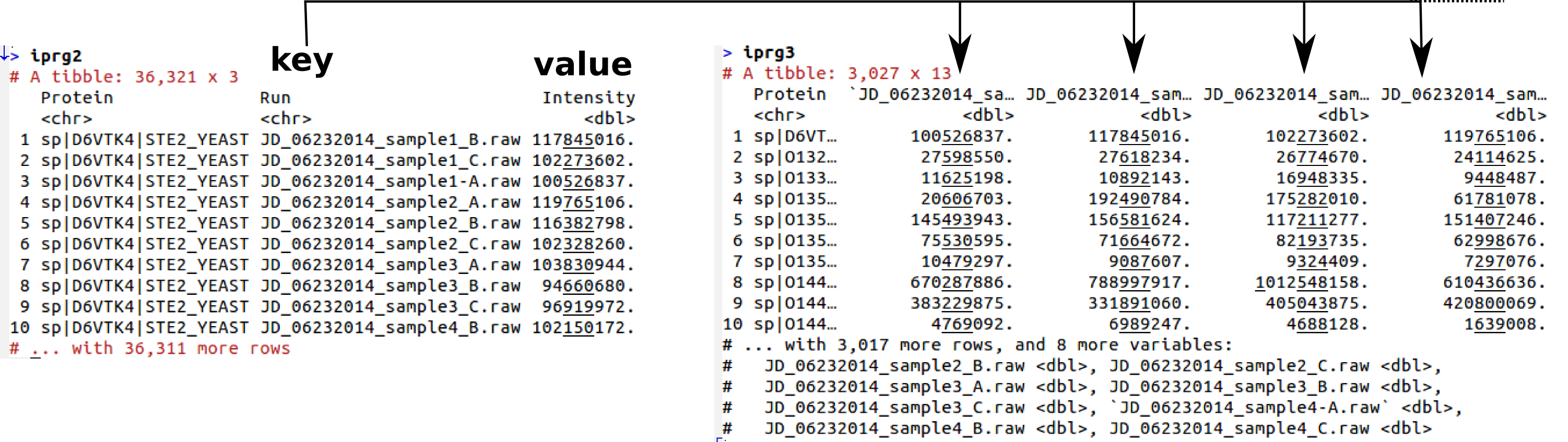
Spreading data from long to wide format
Indeed, we started with
length(unique(iprg$Protein))## [1] 3027unique proteins, which corresponds to the number of rows in the new wide dataset.
The long format is ideal when using ggplot2, as we will see in a later chapter. The wide format has also advantages. For example, it becomes straighforward to verify if there are proteins that haven’t been quantified in some samples.
(k <- which(is.na(iprg3), arr.ind = dim(iprg3)))## row col
## [1,] 2721 2
## [2,] 2721 4
## [3,] 652 11iprg3[unique(k[, "row"]), ]## # A tibble: 2 x 13
## Protein JD_06232014_sam… JD_06232014_sam… `JD_06232014_sa…
## <chr> <dbl> <dbl> <dbl>
## 1 sp|Q08… NA 10989286. NA
## 2 sp|P28… 961274. 1229085. 1108670.
## # … with 9 more variables: JD_06232014_sample2_A.raw <dbl>,
## # JD_06232014_sample2_B.raw <dbl>, JD_06232014_sample2_C.raw <dbl>,
## # JD_06232014_sample3_A.raw <dbl>, JD_06232014_sample3_B.raw <dbl>,
## # JD_06232014_sample3_C.raw <dbl>, JD_06232014_sample4_B.raw <dbl>,
## # JD_06232014_sample4_C.raw <dbl>, `JD_06232014_sample4-A.raw` <dbl>The opposite operation to spread is gather, also from the tidyr package:
(iprg4 <- gather(iprg3, key = Run, value = Intensity, -Protein))## # A tibble: 36,324 x 3
## Protein Run Intensity
## <chr> <chr> <dbl>
## 1 sp|D6VTK4|STE2_YEAST JD_06232014_sample1_B.raw 117845016.
## 2 sp|O13297|CET1_YEAST JD_06232014_sample1_B.raw 27618234.
## 3 sp|O13329|FOB1_YEAST JD_06232014_sample1_B.raw 10892143.
## 4 sp|O13539|THP2_YEAST JD_06232014_sample1_B.raw 192490784.
## 5 sp|O13547|CCW14_YEAST JD_06232014_sample1_B.raw 156581624.
## 6 sp|O13563|RPN13_YEAST JD_06232014_sample1_B.raw 71664672.
## 7 sp|O13585|YP089_YEAST JD_06232014_sample1_B.raw 9087607.
## 8 sp|O14455|RL36B_YEAST JD_06232014_sample1_B.raw 788997917.
## 9 sp|O14467|MBF1_YEAST JD_06232014_sample1_B.raw 331891060.
## 10 sp|O14468|YO304_YEAST JD_06232014_sample1_B.raw 6989247.
## # … with 36,314 more rows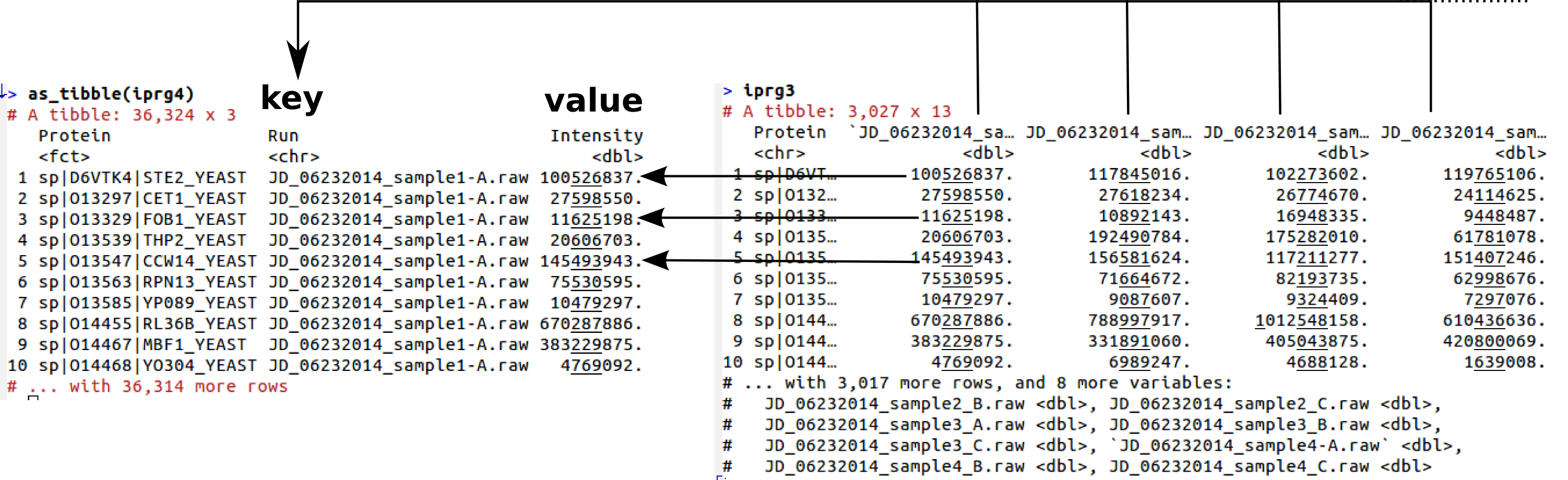
Gathering data from wide to long format
The two lond datasets, iprg2 and iprg4 are different due to the missing values shown above.
nrow(iprg2)## [1] 36321nrow(iprg4)## [1] 36324nrow(na.omit(iprg4))## [1] 36321which can be accounted for by removing rows with missing values by setting na.rm = TRUE.
(iprg5 <- gather(iprg3, key = Run, value = Intensity, -Protein, na.rm = TRUE))## # A tibble: 36,321 x 3
## Protein Run Intensity
## <chr> <chr> <dbl>
## 1 sp|D6VTK4|STE2_YEAST JD_06232014_sample1_B.raw 117845016.
## 2 sp|O13297|CET1_YEAST JD_06232014_sample1_B.raw 27618234.
## 3 sp|O13329|FOB1_YEAST JD_06232014_sample1_B.raw 10892143.
## 4 sp|O13539|THP2_YEAST JD_06232014_sample1_B.raw 192490784.
## 5 sp|O13547|CCW14_YEAST JD_06232014_sample1_B.raw 156581624.
## 6 sp|O13563|RPN13_YEAST JD_06232014_sample1_B.raw 71664672.
## 7 sp|O13585|YP089_YEAST JD_06232014_sample1_B.raw 9087607.
## 8 sp|O14455|RL36B_YEAST JD_06232014_sample1_B.raw 788997917.
## 9 sp|O14467|MBF1_YEAST JD_06232014_sample1_B.raw 331891060.
## 10 sp|O14468|YO304_YEAST JD_06232014_sample1_B.raw 6989247.
## # … with 36,311 more rows2.3 CRC training data
This dataset comes from the MSstatsBioData package and was generated as follows:
library("MSstats")
library("MSstatsBioData")
data(SRM_crc_training)
Quant <- dataProcess(SRM_crc_training)
subjectQuant <- quantification(Quant)
It provides quantitative information for 72 proteins, including two standard proteins, AIAG-Bovine and FETUA-Bovine. These proteins were targeted for plasma samples with SRM with isotope labeled reference peptides in order to identify candidate protein biomarker for non-invasive detection of CRC. The training cohort included 100 subjects in control group and 100 subjects with CRC. Each sample for subject was measured in a single injection without technical replicate. The training cohort was analyzed with Skyline. The dataset was already normalized as described in manuscript. User do not need extra normalization. NAs should be considered as censored missing. Two standard proteins can be removed for statistical analysis.
Clinical information where added manually thereafter.
To load this dataset:
(crcdf <- readr::read_csv("http://bit.ly/VisBiomedDataCrcCsv"))## Parsed with column specification:
## cols(
## .default = col_double(),
## Sample = col_character(),
## Group = col_character(),
## Gender = col_character(),
## Tumour_location = col_character(),
## Sub_group = col_character()
## )## See spec(...) for full column specifications.## # A tibble: 200 x 79
## A1AG2 AFM AHSG `AIAG-Bovine` ANT3 AOC3 APOB ATRN BTD C20orf3
## <dbl> <dbl> <dbl> <dbl> <dbl> <dbl> <dbl> <dbl> <dbl> <dbl>
## 1 14.2 16.1 20.0 15.3 17.2 10.0 15.5 14.4 16.3 10.7
## 2 15.0 16.0 19.7 15.2 17.3 9.04 15.1 14.0 16.2 10.7
## 3 15.6 16.1 19.7 15.6 17.6 10.4 16.0 14.6 16.5 11.2
## 4 15.4 16.3 19.7 15.1 17.4 9.50 15.7 14.1 16.3 9.97
## 5 16.0 17.0 20.4 15.6 18.0 9.65 16.2 14.2 16.5 12.6
## 6 13.9 16.5 19.9 13.4 16.3 9.52 14.5 13.7 15.8 10.6
## 7 14.3 16.4 20.1 15.1 17.4 9.72 14.7 13.3 16.4 11.4
## 8 13.6 17.1 19.9 14.9 17.3 8.79 14.9 12.7 16.1 10.8
## 9 15.8 15.9 18.6 15.1 16.7 8.95 14.7 13.2 15.6 11.6
## 10 15.4 16.2 20.1 15.4 17.6 10.3 15.9 14.7 16.5 11.4
## # … with 190 more rows, and 69 more variables: CADM1 <dbl>, CD163 <dbl>,
## # CD44 <dbl>, CDH5 <dbl>, CFH <dbl>, CFI <dbl>, CLU <dbl>, CP <dbl>,
## # CTSD <dbl>, DKFZp686N02209 <dbl>, DSG2 <dbl>, ECM1 <dbl>, F11 <dbl>,
## # F5 <dbl>, FCGBP <dbl>, `FETUA-Bovine` <dbl>, FETUB <dbl>, FGA <dbl>,
## # FGG <dbl>, FHR3 <dbl>, FN1 <dbl>, GOLM1 <dbl>, HP <dbl>, HRG <dbl>,
## # HYOU1 <dbl>, ICAM1 <dbl>, IGFBP3 <dbl>, IGHA2 <dbl>, IGHG2 <dbl>,
## # ITIH4 <dbl>, KLKB1 <dbl>, KNG1 <dbl>, LAMP2 <dbl>, LCN2 <dbl>,
## # LGALS3BP <dbl>, LRG1 <dbl>, LUM <dbl>, LYVE1 <dbl>, MMRN1 <dbl>,
## # MPO <dbl>, MRC2 <dbl>, MST1 <dbl>, NCAM1 <dbl>, ORM1 <dbl>,
## # PGCP <dbl>, PIGR <dbl>, PLTP <dbl>, PLXDC2 <dbl>, PON1 <dbl>,
## # PRG4 <dbl>, PROC <dbl>, PTPRJ <dbl>, Q5JNX2 <dbl>, SERPINA1 <dbl>,
## # SERPINA3 <dbl>, SERPINA6 <dbl>, SERPINA7 <dbl>, THBS1 <dbl>,
## # TIMP1 <dbl>, TNC <dbl>, VTN <dbl>, VWF <dbl>, Sample <chr>,
## # Group <chr>, Age <dbl>, Gender <chr>, Cancer_stage <dbl>,
## # Tumour_location <chr>, Sub_group <chr>This dataset is in the wide format. It contains the intensity of the proteins in columns 1 to 72 for each of the 200 samples along the rows. Generally, omics datasets contain the features (proteins, transcripts, …) along the rows and the samples along the columns.
In columns 73 to 79, we sample metadata.
crcdf[, 73:79]## # A tibble: 200 x 7
## Sample Group Age Gender Cancer_stage Tumour_location Sub_group
## <chr> <chr> <dbl> <chr> <dbl> <chr> <chr>
## 1 P1A10 CRC 60 female 1 colon CRC
## 2 P1A2 CRC 70 male 1 rectum CRC
## 3 P1A4 CRC 65 male 1 rectum CRC
## 4 P1A6 CRC 65 female 4 colon CRC
## 5 P1B12 CRC 62 female 3 colon CRC
## 6 P1B2 CRC 55 male 2 colon CRC
## 7 P1B3 CRC 61 male 2 rectum CRC
## 8 P1B6 CRC 52 male 4 rectum CRC
## 9 P1B9 CRC 89 female 4 colon CRC
## 10 P1C11 CRC 81 male 1 rectum CRC
## # … with 190 more rowsA widely used data structure for omics data follows the convention described in the figure below:
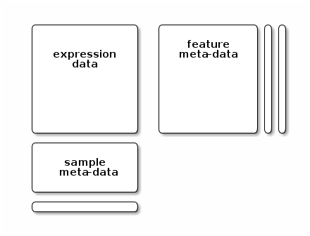
An eSet-type of expression data container
This typical omics data structure, as defined by the eSet class in the Bioconductor Biobase package, is represented below. It’s main features are
An assay data slot containing the quantitative omics data (expression data), stored as a
matrixand accessible withexprs. Features defined along the rows and samples along the columns.A sample metadata slot containing sample co-variates, stored as an annotated
data.frameand accessible withpData. This data frame is stored with rows representing samples and sample covariate along the columns, and its rows match the expression data columns exactly.A feature metadata slot containing feature co-variates, stored as an annotated
data.frameand accessible withfData. This dataframe’s rows match the expression data rows exactly.
The coordinated nature of the high throughput data guarantees that the dimensions of the different slots will always match (i.e the columns in the expression data and then rows in the sample metadata, as well as the rows in the expression data and feature metadata) during data manipulation. The metadata slots can grow additional co-variates (columns) without affecting the other structures.
Below, we show how to transform the crc dataset into an MSnSet (implementing the data structure above for quantitative proteomics data) using the readMSnSet2 function.
library("MSnbase")
i <- 1:72 ## expression columns
e <- t(crcdf[, i]) ## expression data
colnames(e) <- 1:200
crc <- readMSnSet2(data.frame(e), e = 1:200)

pd <- data.frame(crcdf[, -i])
rownames(pd) <- paste0("X", rownames(pd))
pData(crc) <- pd
crc
## MSnSet (storageMode: lockedEnvironment)
## assayData: 72 features, 200 samples
## element names: exprs
## protocolData: none
## phenoData
## sampleNames: X1 X2 ... X200 (200 total)
## varLabels: Sample Group ... Sub_group (7 total)
## varMetadata: labelDescription
## featureData: none
## experimentData: use 'experimentData(object)'
## Annotation:
## - - - Processing information - - -
## MSnbase version: 2.10.0Let’s also set the sample names.
sampleNames(crc) <- crc$SampleTo download and load the MSnSet direcly:
download.file("http://bit.ly/VisBiomedDataCrcMSnSet", "./data/crc.rda")
load("./data/crc.rda")
crc
## MSnSet (storageMode: lockedEnvironment)
## assayData: 72 features, 200 samples
## element names: exprs
## protocolData: none
## phenoData
## sampleNames: P1A10 P1A2 ... P3H6 (200 total)
## varLabels: Sample Group ... Sub_group (7 total)
## varMetadata: labelDescription
## featureData: none
## experimentData: use 'experimentData(object)'
## Annotation:
## - - - Processing information - - -
## MSnbase version: 2.6.0Reference:
See Surinova, S. et al. (2015) Prediction of colorectal cancer diagnosis based on circulating plasma proteins. EMBO Mol. Med., 7, 1166–1178 for details.
2.4 Time course from Mulvey et al. 2015
This data comes from
Mulvey CM, Schröter C, Gatto L, Dikicioglu D, Fidaner IB, Christoforou A, Deery MJ, Cho LT, Niakan KK, Martinez-Arias A, Lilley KS. Dynamic Proteomic Profiling of Extra-Embryonic Endoderm Differentiation in Mouse Embryonic Stem Cells. Stem Cells. 2015 Sep;33(9):2712-25. doi: 10.1002/stem.2067. Epub 2015 Jun 23. PMID: 26059426.
library("pRolocdata")
data(mulvey2015norm)
This MSnSet, available from the pRolocdata package, measured the expression profiles of 2337 proteins along 6 time points in triplicate.
MSnbase::exprs(mulvey2015norm)[1:5, 1:3]## rep1_0hr rep1_16hr rep1_24hr
## P48432 2.479592 1.698630 1.0350877
## Q62315-2 1.979592 1.342466 0.9181287
## P55821 1.780612 1.767123 1.1578947
## P17809 1.637755 1.157534 0.9941520
## Q8K3F7 1.852041 1.623288 1.3040936pData(mulvey2015norm)## rep times cond
## rep1_0hr 1 1 1
## rep1_16hr 1 2 1
## rep1_24hr 1 3 1
## rep1_48hr 1 4 1
## rep1_72hr 1 5 1
## rep1_XEN 1 6 1
## rep2_0hr 2 1 1
## rep2_16hr 2 2 1
## rep2_24hr 2 3 1
## rep2_48hr 2 4 1
## rep2_72hr 2 5 1
## rep2_XEN 2 6 1
## rep3_0hr 3 1 1
## rep3_16hr 3 2 1
## rep3_24hr 3 3 1
## rep3_48hr 3 4 1
## rep3_72hr 3 5 1
## rep3_XEN 3 6 12.5 ALL data
library("ALL")
data(ALL)
ALL
## ExpressionSet (storageMode: lockedEnvironment)
## assayData: 12625 features, 128 samples
## element names: exprs
## protocolData: none
## phenoData
## sampleNames: 01005 01010 ... LAL4 (128 total)
## varLabels: cod diagnosis ... date last seen (21 total)
## varMetadata: labelDescription
## featureData: none
## experimentData: use 'experimentData(object)'
## pubMedIds: 14684422 16243790
## Annotation: hgu95av2From the documentation page:
The Acute Lymphoblastic Leukemia Data from the Ritz Laboratory consist of microarrays from 128 different individuals with acute lymphoblastic leukemia (ALL). A number of additional covariates are available. The data have been normalized (using rma) and it is the jointly normalized data that are available here.
The ALL data is of class ExpressionSet, which implements the data structure above for microarray expression data, and contains normalised and summarised transcript intensities.
Below, we select will patients with B-cell lymphomas and BCR/ABL abnormality and negative controls.
table(ALL$BT)##
## B B1 B2 B3 B4 T T1 T2 T3 T4
## 5 19 36 23 12 5 1 15 10 2table(ALL$mol.biol)##
## ALL1/AF4 BCR/ABL E2A/PBX1 NEG NUP-98 p15/p16
## 10 37 5 74 1 1ALL_bcrneg <- ALL[, ALL$mol.biol %in% c("NEG", "BCR/ABL") & grepl("B", ALL$BT)]
ALL_bcrneg$mol.biol <- factor(ALL_bcrneg$mol.biol)We then use the limma package to
library("limma")
design <- model.matrix(~0+ALL_bcrneg$mol.biol)
colnames(design) <- c("BCR.ABL", "NEG")

## Step1: linear model. lmFit is a wrapper around lm in R
fit1 <- lmFit(ALL_bcrneg, design)

## Step 2: fit contrasts: find genes that respond to estrogen
contrast.matrix <- makeContrasts(BCR.ABL-NEG, levels = design)
fit2 <- contrasts.fit(fit1, contrast.matrix)

## Step3: add empirical Bayes moderation
fit3 <- eBayes(fit2)

## Extract results and set them to the feature data
res <- topTable(fit3, n = Inf)
fData(ALL_bcrneg) <- res[featureNames(ALL_bcrneg), ]
This annotated ExpressionSet can be reproduced as shown above or downloaded and loaded using
download.file("http://bit.ly/VisBiomedDataALL_bcrneg",  "./data/ALL_bcrneg.rda")
load("./data/ALL_bcrneg.rda")
Reference:
Sabina Chiaretti, Xiaochun Li, Robert Gentleman, Antonella Vitale, Marco Vignetti, Franco Mandelli, Jerome Ritz, and Robin Foa Gene expression profile of adult T-cell acute lymphocytic leukemia identifies distinct subsets of patients with different response to therapy and survival. Blood, 1 April 2004, Vol. 103, No. 7.
2.6 Spatial proteomics data
The goal of spatial proteomics is to study the sub-cellular localisation of proteins. The data below comes from
Christoforou A, Mulvey CM, Breckels LM, Geladaki A, Hurrell T, Hayward PC, Naake T, Gatto L, Viner R, Martinez Arias A, Lilley KS. A draft map of the mouse pluripotent stem cell spatial proteome. Nat Commun. 2016 Jan 12;7:8992. doi: 10.1038/ncomms9992. PMID: 26754106; PMCID: PMC4729960.
and investigated the sub-cellular location of over 5000 proteins in mouse pluripotent stem cells using a mass spectrometry-based technique called hyperLOPIT.
library("pRolocdata")
data(hyperLOPIT2015)
dim(hyperLOPIT2015)
## [1] 5032 20In addition to the quantitative data, another important piece of data here are the spatial markers, proteins for which we can confidently assign them a sub-cellular location apriori. These markers are defined in the markers feature variable:
table(fData(hyperLOPIT2015)$markers)##
## 40S Ribosome
## 27
## 60S Ribosome
## 43
## Actin cytoskeleton
## 13
## Cytosol
## 43
## Endoplasmic reticulum/Golgi apparatus
## 107
## Endosome
## 13
## Extracellular matrix
## 13
## Lysosome
## 33
## Mitochondrion
## 383
## Nucleus - Chromatin
## 64
## Nucleus - Non-chromatin
## 85
## Peroxisome
## 17
## Plasma membrane
## 51
## Proteasome
## 34
## unknown
## 4106Here, the columns of the data represent fractions along a density gradient used to separate the sub-cellular proteome presented in this data.
We will be using a simplified version of this data in the next chapters. Below, we retain the first replicate (hyperLOPIT2015$Replicate == 1]) and the marker proteins (using the markerMSnSet function):
hlm <- pRoloc::markerMSnSet(hyperLOPIT2015[, hyperLOPIT2015$Replicate == 1])
dim(hlm)
## [1] 926 10getMarkerClasses(hlm) ## no unknowns anymore## [1] "40S Ribosome"
## [2] "60S Ribosome"
## [3] "Actin cytoskeleton"
## [4] "Cytosol"
## [5] "Endoplasmic reticulum/Golgi apparatus"
## [6] "Endosome"
## [7] "Extracellular matrix"
## [8] "Lysosome"
## [9] "Mitochondrion"
## [10] "Nucleus - Chromatin"
## [11] "Nucleus - Non-chromatin"
## [12] "Peroxisome"
## [13] "Plasma membrane"
## [14] "Proteasome"