Machine learning techniques available in pRoloc

Laurent Gatto

de Duve Institute, UCLouvain, Belgium

Abstract

This vignette provides a general background about machine learning (ML) methods and concepts, and their application to the analysis of spatial proteomics data in the pRoloc package. See the pRoloc-tutorial vignette for details about the package itself.

Introduction

For a general practical introduction to pRoloc, readers are referred to the tutorial, available using vignette("pRoloc-tutorial", package = "pRoloc"). The following document provides a overview of the algorithms available in the package. The respective section describe unsupervised machine learning (USML), supervised machine learning (SML), semi-supervised machine learning (SSML) as implemented in the novelty detection algorithm and transfer learning.

Data sets

We provide 144 test data sets in the pRolocdata package that can be readily used with pRoloc. The data set can be listed with pRolocdata and loaded with the data function. Each data set, including its origin, is individually documented.

The data sets are distributed as MSnSet instances. Briefly, these are dedicated containers for quantitation data as well as feature and sample meta-data. More details about MSnSets are available in the pRoloc tutorial and in the MSnbase package, that defined the class.

library("pRolocdata")
data(tan2009r1)
tan2009r1

## MSnSet (storageMode: lockedEnvironment)
## assayData: 888 features, 4 samples 
##   element names: exprs 
## protocolData: none
## phenoData
##   sampleNames: X114 X115 X116 X117
##   varLabels: Fractions
##   varMetadata: labelDescription
## featureData
##   featureNames: P20353 P53501 ... P07909 (888 total)
##   fvarLabels: FBgn Protein.ID ... markers.tl (16 total)
##   fvarMetadata: labelDescription
## experimentData: use 'experimentData(object)'
##   pubMedIds: 19317464 
## Annotation:  
## - - - Processing information - - -
## Added markers from  'mrk' marker vector. Thu Jul 16 22:53:44 2015 
##  MSnbase version: 1.17.12

Other omics data

While our primary biological domain is quantitative proteomics, with special emphasis on spatial proteomics, the underlying class infrastructure on which pRoloc and implemented in the Bioconductor MSnbase package enables the conversion from/to transcriptomics data, in particular microarray data available as ExpressionSet objects using the as coercion methods (see the MSnSet section in the MSnbase-development vignette). As a result, it is straightforward to apply the methods summarised here in detailed in the other pRoloc vignettes to these other data structures.

Unsupervised machine learning

Unsupervised machine learning refers to clustering, i.e. finding structure in a quantitative, generally multi-dimensional data set of unlabelled data.

Currently, unsupervised clustering facilities are available through the plot2D function and the MLInterfaces package (Carey et al., n.d.). The former takes an MSnSet instance and represents the data on a scatter plot along the first two principal components. Arbitrary feature meta-data can be represented using different colours and point characters. The reader is referred to the manual page available through ?plot2D for more details and examples.

pRoloc also implements a MLean method for MSnSet instances, allowing to use the relevant infrastructure with the organelle proteomics framework. Although provides a common interface to unsupervised and numerous supervised algorithms, we refer to the pRoloc tutorial for its usage to several clustering algorithms.

Note Current development efforts in terms of clustering are described on the Clustering infrastructure wiki page (https://github.com/lgatto/pRoloc/wiki/Clustering-infrastructure) and will be incorporated in future version of the package.

Supervised machine learning

Supervised machine learning refers to a broad family of classification algorithms. The algorithms learns from a modest set of labelled data points called the training data. Each training data example consists of a pair of inputs: the actual data, generally represented as a vector of numbers and a class label, representing the membership to exactly 1 of multiple possible classes. When there are only two possible classes, on refers to binary classification. The training data is used to construct a model that can be used to classifier new, unlabelled examples. The model takes the numeric vectors of the unlabelled data points and return, for each of these inputs, the corresponding mapped class.

Algorithms used

k-nearest neighbour (KNN) Function knn from package class. For each row of the test set, the k nearest (in Euclidean distance) training set vectors are found, and the classification is decided by majority vote over the k classes, with ties broken at random. This is a simple algorithm that is often used as baseline classifier. If there are ties for the kth nearest vector, all candidates are included in the vote.

Partial least square DA (PLS-DA) Function plsda from package . Partial least square discriminant analysis is used to fit a standard PLS model for classification.

Support vector machine (SVM) A support vector machine constructs a hyperplane (or set of hyperplanes for multiple-class problem), which are then used for classification. The best separation is defined as the hyperplane that has the largest distance (the margin) to the nearest data points in any class, which also reduces the classification generalisation error. To assure liner separation of the classes, the data is transformed using a kernel function into a high-dimensional space, permitting liner separation of the classes.

pRoloc makes use of the functions svm from package and ksvm from .

Artificial neural network (ANN) Function nnet from package . Fits a single-hidden-layer neural network, possibly with skip-layer connections.

Naive Bayes (NB) Function naiveBayes from package . Naive Bayes classifier that computes the conditional a-posterior probabilities of a categorical class variable given independent predictor variables using the Bayes rule. Assumes independence of the predictor variables, and Gaussian distribution (given the target class) of metric predictors.

Random Forest (RF) Function randomForest from package .

Chi-square ($\chi^2$) Assignment based on squared differences between a labelled marker and a new feature to be classified. Canonical protein correlation profile method (PCP) uses squared differences between a labelled marker and new features. In (Andersen et al. 2003), $\chi^2$ is defined as , i.e. $\chi^{2} = \frac{\sum_{i=1}^{n} (x_i - m_i)^{2}}{n}$, whereas (Wiese et al. 2007) divide by the value the squared value by the value of the reference feature in each fraction, i.e. $\chi^{2} = \sum_{i=1}^{n}\frac{(x_i - m_i)^{2}}{m_i}$, where $x_i$ is normalised intensity of feature x in fraction i, $m_i$ is the normalised intensity of marker m in fraction i and n is the number of fractions available. We will use the former definition.

PerTurbo From (Courty, Burger, and Laurent 2011): PerTurbo, an original, non-parametric and efficient classification method is presented here. In our framework, the manifold of each class is characterised by its Laplace-Beltrami operator, which is evaluated with classical methods involving the graph Laplacian. The classification criterion is established thanks to a measure of the magnitude of the spectrum perturbation of this operator. The first experiments show good performances against classical algorithms of the state-of-the-art. Moreover, from this measure is derived an efficient policy to design sampling queries in a context of active learning. Performances collected over toy examples and real world datasets assess the qualities of this strategy.

The PerTurbo implementation comes from the pRoloc packages.

Estimating algorithm parameters

It is essential when applying any of the above classification algorithms, to wisely set the algorithm parameters, as these can have an important effect on the classification. Such parameters are for example the width sigma of the Radial Basis Function (Gaussian kernel) $exp(-\sigma \| x - x' \|^2 )$ and the cost (slack) parameter (controlling the tolerance to mis-classification) of our SVM classifier. The number of neighbours k of the KNN classifier is equally important as will be discussed in this sections.

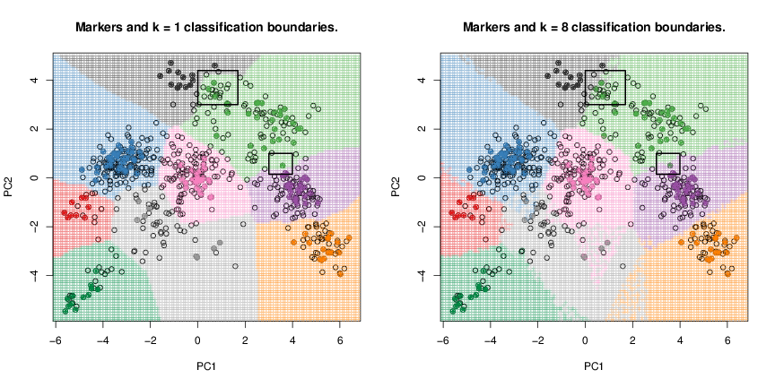
The next figure illustrates the effect of different choices of $k$ using organelle proteomics data from (Dunkley et al. 2006) (dunkley2006 from pRolocdata). As highlighted in the squared region, we can see that using a low $k$ (k = 1 on the left) will result in very specific classification boundaries that precisely follow the contour or our marker set as opposed to a higher number of neighbours (k = 8 on the right). While one could be tempted to believe that optimised classification boundaries are preferable, it is essential to remember that these boundaries are specific to the marker set used to construct them, while there is absolutely no reason to expect these regions to faithfully separate any new data points, in particular proteins that we wish to classify to an organelle. In other words, the highly specific k = 1 classification boundaries are over-fitted for the marker set or, in other words, lack generalisation to new instances. We will demonstrate this using simulated data taken from (James et al. 2013) and show what detrimental effect over-fitting has on new data.

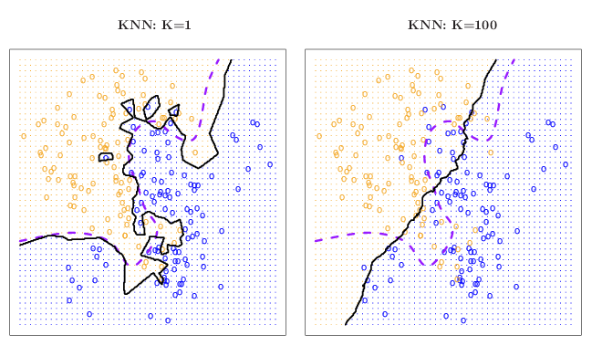
Classification boundaries using $k=1$ or $k=8$ on the dunkley2006 data.

The figure below uses 2 x 100 simulated data points belonging to either of the orange or blue classes. The genuine classes for all the points is known (solid lines) and the KNN algorithm has been applied using k = 1 (left) and k = 100 (right) respectively (purple dashed lines). As in our organelle proteomics examples, we observe that when k = 1, the decision boundaries are overly flexible and identify patterns in the data that do not reflect to correct boundaries (in such cases, the classifier is said to have low bias but very high variance). When a large k is used, the classifier becomes inflexible and produces approximate and nearly linear separation boundaries (such a classifier is said to have low variance but high bias). On this simulated data set, neither k = 1 nor k = 100 give good predictions and have test error rates (i.e. the proportion of wrongly classified points) of 0.1695 and 0.1925, respectively.

The KNN classifier using $k = 1$ (left, solid classification boundaries) and $k = 100$ (right, solid classification boundaries) compared the Bayes decision boundaries (see original material for details). Reproduced with permission from (James et al. 2013).

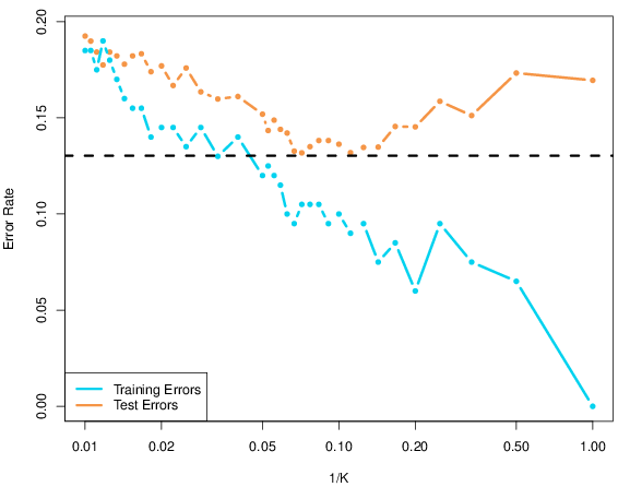
To quantify the effect of flexibility and lack thereof in defining the classification boundaries, (James et al. 2013) calculate the classification error rates using training data (training error rate) and testing data (testing error rate). The latter is completely new data that was not used to assess the model error rate when defining algorithm parameters; one often says that the model used for classification has not seen this data. If the model performs well on new data, it is said to generalise well. This is a quality that is required in most cases, and in particular in our organelle proteomics experiments where the training data corresponds to our marker sets. Figure @ref{fig:ISL2} plots the respective training and testing error rates as a function of 1/k which is a reflection of the flexibility/complexity of our model; when 1/k = 1, i.e. k = 1 (far right), we have a very flexible model with the risk of over-fitting. Greater values of k (towards the left) characterise less flexible models. As can be seen, high values of k produce poor performance for both training and testing data. However, while the training error steadily decreases when the model complexity increases (smaller k), the testing error rate displays a typical U-shape: at a value around k = 10, the testing error rate reaches a minimum and then starts to increase due to over-fitting to the training data and lack of generalisation of the model.

Effect of train and test error with respect to model complexity. The former decreases for lower values of $k$ while the test error reaches a minimum around $k = 10$ before increasing again. Reproduced with permission from (James et al. 2013).

These results show that adequate optimisation of the model parameters are essential to avoid either too flexible models (that do not generalise well to new data) or models that do not describe the decision boundaries adequately. Such parameter selection is achieved by cross validation, where the initial marker proteins are separated into training data used to build classification models and independent testing data used to assess the model on new data.

We recommend the book An Introduction to Statistical Learning (http://www-bcf.usc.edu/~gareth/ISL/) by (James et al. 2013) for a more detailed introduction of machine learning.

Default analysis scheme

Below, we present a typical classification analysis using pRoloc. The analysis typically consists of two steps. The first one is to optimise the classifier parameters to be used for training and testing (see above). A range of parameters are tested using the labelled data, for which the labels are known. For each set of parameters, we hide the labels of a subset of labelled data and use the other part to train a model and apply in on the testing data with hidden labels. The comparison of the estimated and expected labels enables to assess the validity of the model and hence the adequacy if the parameters. Once adequate parameters have been identified, they are used to infer a model on the complete organelle marker set and used to infer the sub-cellular location of the unlabelled examples.

Parameter optimisation

Algorithmic performance is estimated using a stratified 20/80 partitioning. The 80% partitions are subjected to 5-fold cross-validation in order to optimise free parameters via a grid search, and these parameters are then applied to the remaining 20%. The procedure is repeated n = 100 times to sample n accuracy metrics (see below) values using n, possibly different, optimised parameters for evaluation.

Models accuracy is evaluated using the F1 score, $F1 = 2 ~ \frac{precision \times recall}{precision + recall}$, calculated as the harmonic mean of the precision ($precision = \frac{tp}{tp+fp}$, a measure of exactness – returned output is a relevant result) and recall ($recall=\frac{tp}{tp+fn}$, a measure of completeness – indicating how much was missed from the output). What we are aiming for are high generalisation accuracy, i.e high $F1$, indicating that the marker proteins in the test data set are consistently correctly assigned by the algorithms.

The results of the optimisation procedure are stored in an GenRegRes object that can be inspected, plotted and best parameter pairs can be extracted.

For a given algorithm alg, the corresponding parameter optimisation function is names algOptimisation or, equivalently, algOptimization. See the table below for details. A description of each of the respective model parameters is provided in the optimisation function manuals, available through ?algOptimisation.

params <- svmOptimisation(tan2009r1, times = 10,
                          xval = 5, verbose = FALSE)
params

## Object of class "GenRegRes"
## Algorithm: svm 
## Hyper-parameters:
##  cost: 0.0625 0.125 0.25 0.5 1 2 4 8 16
##  sigma: 0.001 0.01 0.1 1 10 100
## Design:
##  Replication: 10 x 5-fold X-validation
##  Partitioning: 0.2/0.8 (test/train)
## Results
##  macro F1:
##    Min. 1st Qu.  Median    Mean 3rd Qu.    Max. 
##  0.7804  0.8085  0.8211  0.8412  0.8842  0.9385 
##  best sigma: 0.1 1   
##  best cost: 8 16 2 1   
## Use getWarnings() to see warnings.

Classification

tan2009r1 <- svmClassification(tan2009r1, params)

## [1] "markers"

tan2009r1

## MSnSet (storageMode: lockedEnvironment)
## assayData: 888 features, 4 samples 
##   element names: exprs 
## protocolData: none
## phenoData
##   sampleNames: X114 X115 X116 X117
##   varLabels: Fractions
##   varMetadata: labelDescription
## featureData
##   featureNames: P20353 P53501 ... P07909 (888 total)
##   fvarLabels: FBgn Protein.ID ... svm.scores (18 total)
##   fvarMetadata: labelDescription
## experimentData: use 'experimentData(object)'
##   pubMedIds: 19317464 
## Annotation:  
## - - - Processing information - - -
## Added markers from  'mrk' marker vector. Thu Jul 16 22:53:44 2015 
## Performed svm prediction (sigma=1 cost=2) Sat Nov 23 16:06:33 2024 
##  MSnbase version: 1.17.12

Customising model parameters

Below we illustrate how to weight different classes according to the number of labelled instances, where large sets are down weighted. This strategy can help with imbalanced designs.

w <- table(fData(markerMSnSet(dunkley2006))$markers)
wpar <- svmOptimisation(dunkley2006, class.weights = w)
wres <- svmClassification(dunkley2006, wpar, class.weights = w)

parameter optimisation	classification	algorithm	package
knnOptimisation	knnClassification	nearest neighbour	class
knntlOptimisation	knntlClassification	nearest neighbour transfer learning	pRoloc
ksvmOptimisation	ksvmClassification	support vector machine	kernlab
nbOptimisation	nbClassification	naive bayes	e1071
nnetOptimisation	nnetClassification	neural networks	nnet
perTurboOptimisation	perTurboClassification	PerTurbo	pRoloc
plsdaOptimisation	plsdaClassification	partial least square	caret
rfOptimisation	rfClassification	random forest	randomForest
svmOptimisation	svmClassification	support vector machine	e1071

Comparison of different classifiers

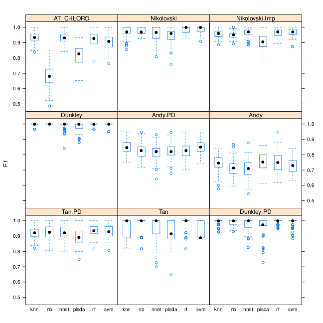
Several supervised machine learning algorithms have already been applied to organelle proteomics data classification: partial least square discriminant analysis in (Dunkley et al. 2006, Tan2009), support vector machines (SVMs) in (Trotter et al. 2010), random forest in (Ohta et al. 2010), neural networks in (Tardif et al. 2012), naive Bayes (Nikolovski et al. 2012). In our HUPO 2011 poster¹, we show that different classification algorithms provide very similar performance. We have extended this comparison on various datasets distributed in the pRolocdata package. On figure @ref{fig:f1box}, we illustrate how different algorithms reach very similar performances on most of our test datasets.

Comparison of classification performances of several contemporary classification algorithms on data from the pRolocdata package.

Bayesian generative models

We also offer generative models that, as opposed to the descriptive classifier presented above, explicitly model the spatial proteomics data. In pRoloc, we probose two models using T-augmented Gaussian mixtures using repectively a Expectration-Maximisation approach to maximum a posteriori estimation of the model parameters (TAGM-MAP), and an MCMC approach (TAGM-MCMC) that enables a proteome-wide uncertainty quantitation. These methods are described in the pRoloc-bayesian vignette.

For a details description of the methods and their validation, please refer to (Crook et al. 2018):

A Bayesian Mixture Modelling Approach For Spatial Proteomics Oliver M Crook, Claire M Mulvey, Paul D. W. Kirk, Kathryn S Lilley, Laurent Gatto bioRxiv 282269; doi: https://doi.org/10.1101/282269

Semi-supervised machine learning

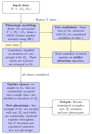
The phenoDisco algorithm is a semi-supervised novelty detection method by (Lisa M. Breckels et al. 2013) (figure below). It uses the labelled (i.e. markers, noted $D_L$) and unlabelled (i.e. proteins of unknown localisation, noted $D_U$) sets of the input data. The algorithm is repeated $N$ times (the times argument in the phenoDisco function). At each iteration, each organelle class $D_{L}^{i}$ and the unlabelled complement are clustered using Gaussian mixture modelling. While unlabelled members that systematically cluster with $D_{L}^{i}$ and pass outlier detection are labelled as new putative members of class $i$, any example of $D_U$ which are not merged with any any of the $D_{L}^{i}$ and are consistently clustered together throughout the $N$ iterations are considered members of a new phenotype.

The PhenoDisco iterative algorithm.

Transfer learning

When multiple sources of data are available, it is often beneficial to take all or several into account with the aim of increasing the information to tackle a problem of interest. While it is at times possible to combine these different sources of data, this can lead to substantially harm to performance of the analysis when the different data sources are of variable signal-to-noise ratio or the data are drawn from different domains and recorded by different encoding (quantitative and binary, for example). If we defined the following two data source

1. primary data, of high signal-to-noise ratio, but general available in limited amounts;
2. auxiliary data, of limited signal-to-noise, and available in large amounts;

then, a transfer learning algorithm will efficiently support/complement the primary target domain with auxiliary data features without compromising the integrity of our primary data.

We have developed a transfer learning framework (L. M. Breckels et al. 2016) and applied to the analysis of spatial proteomics data, as described in the pRoloc-transfer-learning vignette.

Session information

All software and respective versions used to produce this document are listed below.

## R Under development (unstable) (2024-11-20 r87352)
## Platform: x86_64-pc-linux-gnu
## Running under: Ubuntu 24.04.1 LTS
## 
## Matrix products: default
## BLAS:   /usr/lib/x86_64-linux-gnu/openblas-pthread/libblas.so.3 
## LAPACK: /usr/lib/x86_64-linux-gnu/openblas-pthread/libopenblasp-r0.3.26.so;  LAPACK version 3.12.0
## 
## locale:
##  [1] LC_CTYPE=en_US.UTF-8       LC_NUMERIC=C              
##  [3] LC_TIME=en_US.UTF-8        LC_COLLATE=en_US.UTF-8    
##  [5] LC_MONETARY=en_US.UTF-8    LC_MESSAGES=en_US.UTF-8   
##  [7] LC_PAPER=en_US.UTF-8       LC_NAME=C                 
##  [9] LC_ADDRESS=C               LC_TELEPHONE=C            
## [11] LC_MEASUREMENT=en_US.UTF-8 LC_IDENTIFICATION=C       
## 
## time zone: UTC
## tzcode source: system (glibc)
## 
## attached base packages:
## [1] stats4    stats     graphics  grDevices utils     datasets  methods  
## [8] base     
## 
## other attached packages:
##  [1] pRolocdata_1.45.1    pRoloc_1.47.1        BiocParallel_1.41.0 
##  [4] MLInterfaces_1.87.0  cluster_2.1.6        annotate_1.85.0     
##  [7] XML_3.99-0.17        AnnotationDbi_1.69.0 IRanges_2.41.1      
## [10] MSnbase_2.33.2       ProtGenerics_1.39.0  S4Vectors_0.45.2    
## [13] mzR_2.41.1           Rcpp_1.0.13-1        Biobase_2.67.0      
## [16] BiocGenerics_0.53.3  generics_0.1.3       knitr_1.49          
## [19] BiocStyle_2.35.0    
## 
## loaded via a namespace (and not attached):
##   [1] splines_4.5.0               filelock_1.0.3             
##   [3] tibble_3.2.1                hardhat_1.4.0              
##   [5] preprocessCore_1.69.0       pROC_1.18.5                
##   [7] rpart_4.1.23                lifecycle_1.0.4            
##   [9] httr2_1.0.6                 doParallel_1.0.17          
##  [11] globals_0.16.3              lattice_0.22-6             
##  [13] MASS_7.3-61                 MultiAssayExperiment_1.33.1
##  [15] dendextend_1.19.0           magrittr_2.0.3             
##  [17] limma_3.63.2                plotly_4.10.4              
##  [19] sass_0.4.9                  rmarkdown_2.29             
##  [21] jquerylib_0.1.4             yaml_2.3.10                
##  [23] MsCoreUtils_1.19.0          DBI_1.2.3                  
##  [25] RColorBrewer_1.1-3          lubridate_1.9.3            
##  [27] abind_1.4-8                 zlibbioc_1.53.0            
##  [29] GenomicRanges_1.59.1        purrr_1.0.2                
##  [31] mixtools_2.0.0              AnnotationFilter_1.31.0    
##  [33] nnet_7.3-19                 rappdirs_0.3.3             
##  [35] ipred_0.9-15                lava_1.8.0                 
##  [37] GenomeInfoDbData_1.2.13     listenv_0.9.1              
##  [39] gdata_3.0.1                 parallelly_1.39.0          
##  [41] pkgdown_2.1.1.9000          ncdf4_1.23                 
##  [43] codetools_0.2-20            DelayedArray_0.33.2        
##  [45] xml2_1.3.6                  tidyselect_1.2.1           
##  [47] UCSC.utils_1.3.0            viridis_0.6.5              
##  [49] matrixStats_1.4.1           BiocFileCache_2.15.0       
##  [51] jsonlite_1.8.9              caret_6.0-94               
##  [53] e1071_1.7-16                survival_3.7-0             
##  [55] iterators_1.0.14            systemfonts_1.1.0          
##  [57] foreach_1.5.2               segmented_2.1-3            
##  [59] tools_4.5.0                 progress_1.2.3             
##  [61] ragg_1.3.3                  glue_1.8.0                 
##  [63] prodlim_2024.06.25          gridExtra_2.3              
##  [65] SparseArray_1.7.2           xfun_0.49                  
##  [67] MatrixGenerics_1.19.0       GenomeInfoDb_1.43.1        
##  [69] dplyr_1.1.4                 withr_3.0.2                
##  [71] BiocManager_1.30.25         fastmap_1.2.0              
##  [73] fansi_1.0.6                 digest_0.6.37              
##  [75] timechange_0.3.0            R6_2.5.1                   
##  [77] textshaping_0.4.0           colorspace_2.1-1           
##  [79] gtools_3.9.5                lpSolve_5.6.22             
##  [81] biomaRt_2.63.0              RSQLite_2.3.8              
##  [83] utf8_1.2.4                  tidyr_1.3.1                
##  [85] hexbin_1.28.5               data.table_1.16.2          
##  [87] recipes_1.1.0               FNN_1.1.4.1                
##  [89] class_7.3-22                prettyunits_1.2.0          
##  [91] PSMatch_1.11.0              httr_1.4.7                 
##  [93] htmlwidgets_1.6.4           S4Arrays_1.7.1             
##  [95] ModelMetrics_1.2.2.2        pkgconfig_2.0.3            
##  [97] gtable_0.3.6                timeDate_4041.110          
##  [99] blob_1.2.4                  impute_1.81.0              
## [101] XVector_0.47.0              htmltools_0.5.8.1          
## [103] bookdown_0.41               MALDIquant_1.22.3          
## [105] clue_0.3-66                 scales_1.3.0               
## [107] png_0.1-8                   gower_1.0.1                
## [109] reshape2_1.4.4              coda_0.19-4.1              
## [111] nlme_3.1-166                curl_6.0.1                 
## [113] proxy_0.4-27                cachem_1.1.0               
## [115] stringr_1.5.1               parallel_4.5.0             
## [117] mzID_1.45.0                 vsn_3.75.0                 
## [119] desc_1.4.3                  pillar_1.9.0               
## [121] grid_4.5.0                  vctrs_0.6.5                
## [123] pcaMethods_1.99.0           randomForest_4.7-1.2       
## [125] dbplyr_2.5.0                xtable_1.8-4               
## [127] evaluate_1.0.1              mvtnorm_1.3-2              
## [129] cli_3.6.3                   compiler_4.5.0             
## [131] rlang_1.1.4                 crayon_1.5.3               
## [133] future.apply_1.11.3         LaplacesDemon_16.1.6       
## [135] mclust_6.1.1                QFeatures_1.17.0           
## [137] affy_1.85.0                 plyr_1.8.9                 
## [139] fs_1.6.5                    stringi_1.8.4              
## [141] viridisLite_0.4.2           munsell_0.5.1              
## [143] Biostrings_2.75.1           lazyeval_0.2.2             
## [145] Matrix_1.7-1                hms_1.1.3                  
## [147] bit64_4.5.2                 future_1.34.0              
## [149] ggplot2_3.5.1               KEGGREST_1.47.0            
## [151] statmod_1.5.0               SummarizedExperiment_1.37.0
## [153] kernlab_0.9-33              igraph_2.1.1               
## [155] memoise_2.0.1               affyio_1.77.0              
## [157] bslib_0.8.0                 sampling_2.10              
## [159] bit_4.5.0

References

Andersen, Jens S., Christopher J. Wilkinson, Thibault Mayor, Peter Mortensen, Erich A. Nigg, and Matthias Mann. 2003. “Proteomic Characterization of the Human Centrosome by Protein Correlation Profiling.” Nature 426 (6966): 570–74. https://doi.org/10.1038/nature02166.

Breckels, L M, S B Holden, D Wojnar, C M Mulvey, A Christoforou, A Groen, M W Trotter, O Kohlbacher, K S Lilley, and L Gatto. 2016. “Learning from Heterogeneous Data Sources: An Application in Spatial Proteomics.” PLoS Comput Biol 12 (5): e1004920. https://doi.org/10.1371/journal.pcbi.1004920.

Breckels, Lisa M, Laurent Gatto, Andy Christoforou, Arnoud J Groen, Kathryn S Lilley, and Matthew W B Trotter. 2013. “The Effect of Organelle Discovery Upon Sub-Cellular Protein Localisation.” J Proteomics, March. https://doi.org/10.1016/j.jprot.2013.02.019.

Carey, Vince, Robert Gentleman, Jess Mar, and contributions from Jason Vertrees, and Laurent Gatto. n.d. MLInterfaces: Uniform Interfaces to r Machine Learning Procedures for Data in Bioconductor Containers.

Courty, Nicolas, Thomas Burger, and Johann Laurent. 2011. “PerTurbo: A New Classification Algorithm Based on the Spectrum Perturbations of the Laplace-Beltrami Operator.” In In the Proceedings of ECML/PKDD (1), edited by Dimitrios Gunopulos, Thomas Hofmann, Donato Malerba, and Michalis Vazirgiannis, 6911:359–74. Lecture Notes in Computer Science. Springer.

Crook, Oliver M, Claire M Mulvey, Paul D. W. Kirk, Kathryn S Lilley, and Laurent Gatto. 2018. “A Bayesian Mixture Modelling Approach for Spatial Proteomics.” bioRxiv. https://doi.org/10.1101/282269.

Dunkley, Tom P. J., Svenja Hester, Ian P. Shadforth, John Runions, Thilo Weimar, Sally L. Hanton, Julian L. Griffin, et al. 2006. “Mapping the Arabidopsis Organelle Proteome.” Proc Natl Acad Sci USA 103 (17): 6518–23. https://doi.org/10.1073/pnas.0506958103.

James, G., D. Witten, T. Hastie, and R. Tibshirani. 2013. An Introduction to Statistical Learning: With Applications in r. Springer Texts in Statistics. Springer.

Nikolovski, N, D Rubtsov, M P Segura, G P Miles, T J Stevens, T P Dunkley, S Munro, K S Lilley, and P Dupree. 2012. “Putative Glycosyltransferases and Other Plant Golgi Apparatus Proteins Are Revealed by LOPIT Proteomics.” Plant Physiol 160 (2): 1037–51. https://doi.org/10.1104/pp.112.204263.

Ohta, S, J C Bukowski-Wills, L Sanchez-Pulido, Fde L Alves, L Wood, Z A Chen, M Platani, et al. 2010. “The Protein Composition of Mitotic Chromosomes Determined Using Multiclassifier Combinatorial Proteomics.” Cell 142 (5): 810–21. https://doi.org/10.1016/j.cell.2010.07.047.

Tardif, M, A Atteia, M Specht, G Cogne, N Rolland, S Brugière, M Hippler, et al. 2012. “PredAlgo: A New Subcellular Localization Prediction Tool Dedicated to Green Algae.” Mol Biol Evol 29 (12): 3625–39. https://doi.org/10.1093/molbev/mss178.

Trotter, Matthew W. B., Pawel G. Sadowski, Tom P. J. Dunkley, Arnoud J. Groen, and Kathryn S. Lilley. 2010. “Improved Sub-Cellular Resolution via Simultaneous Analysis of Organelle Proteomics Data Across Varied Experimental Conditions.” PROTEOMICS 10 (23): 4213–19. https://doi.org/10.1002/pmic.201000359.

Wiese, Sebastian, Thomas Gronemeyer, Rob Ofman, Markus Kunze, Cláudia P. Grou, José A. Almeida, Martin Eisenacher, et al. 2007. “Proteomics Characterization of Mouse Kidney Peroxisomes by Tandem Mass Spectrometry and Protein Correlation Profiling.” Mol Cell Proteomics 6 (12): 2045–57. https://doi.org/10.1074/mcp.M700169-MCP200.