Fragment matching using synapter

Laurent Gatto

Computational Proteomics Unit, Cambridge, UK.

Sebastian Gibb

Department of Anesthesiology and Intensive Care, University Medicine Greifswald, Germany.

Pavel V. Shliaha

Department of Biochemistry and Molecular Biology, University of Southern Denmark, Denmark.

Abstract

This vignette describes how to apply fragment matching to MS\(^E\)/HDMS\(^E\) data using the ‘synapter’ package. The fragment matching feature allows one to rescue non unique matches and remove falsely assigned unique matches as well.

Foreword

synapter is free and open-source software. If you use it, please support the project by citing it in publications:

Nicholas James Bond, Pavel Vyacheslavovich Shliaha, Kathryn S. Lilley, and Laurent Gatto. Improving qualitative and quantitative performance for MS\(^E\)-based label free proteomics. J. Proteome Res., 2013, 12 (6), pp 2340–2353

Questions and bugs

For bugs, typos, suggestions or other questions, please file an issue in our tracking system (https://github.com/lgatto/synapter/issues) providing as much information as possible, a reproducible example and the output of sessionInfo().

If you don’t have a GitHub account or wish to reach a broader audience for general questions about proteomics analysis using R, you may want to use the Bioconductor support site: https://support.bioconductor.org/.

Introduction

This document assumes familiarity with standard synapter pipeline described in (Bond et al. 2013) and in the package synapter vignette, available online and with vignette("synapter", package = "synapter").

In this vignette we introduce a new fragment matching feature (see figures 2, 3 and 4) which improves the matching of identification and the quantitation features. After applying the usual synergise1 workflow (see ?synergise1 and ?Synapter for details) a number of multiple matches and possible false unique matches remain that can be deconvoluted by comparing common peaks in the identification fragment peaks and the quantitation spectra.

The example data synobj2 used throughout this document is available in the synapterdata package and can be directly load as follows:

library("synapterdata")
synobj2RData()

In the [next section](:synergise] we describe how synobj2 was generated. The test files used in this vignette can be downloaded from http://proteome.sysbiol.cam.ac.uk/lgatto/synapter/data/. The following sections then describe the new fragment matching functionality.

Running synergise1

One has to run the synergise1 workflow before fragment matching can be applied. Please read the general synapter vignette for the general use of synergise1. The additional data needed for the fragment matching procedure are a final_fragment.csv file for the identification run and a Spectrum.xml file for the quantitation run.

## Please find the raw data at:
## http://proteome.sysbiol.cam.ac.uk/lgatto/synapter/data/
library("synapter")

inlist <- list(
  identpeptide = "fermentor_03_sample_01_HDMSE_01_IA_final_peptide.csv.gz",
  identfragments = "fermentor_03_sample_01_HDMSE_01_IA_final_fragment.csv.gz",
  quantpeptide = "fermentor_02_sample_01_HDMSE_01_IA_final_peptide.csv.gz",
  quantpep3d = "fermentor_02_sample_01_HDMSE_01_Pep3DAMRT.csv.gz",
  quantspectra = "fermentor_02_sample_01_HDMSE_01_Pep3D_Spectrum.xml.gz",
  fasta = "S.cerevisiae_Uniprot_reference_canonical_18_03_14.fasta")

synobj2 <- Synapter(inlist, master=FALSE)

synobj2 <- synergise1(object=synobj2,
                      outputdir=tempdir())

Filtering fragments

This step is optional and allows one to remove low abundance fragments in the spectra using filterFragments. Filtering fragments can remove noise in the spectra and reduce undesired fragment matches. Prior to filtering, the plotCumulativeNumberOfFragments function can be use to visualise the intensity of all fragments. Both functions have an argument what to decide what spectra/fragments to filter/plot. Choose fragments.ident for the identification fragments and spectra.quant for the quantitation fragments.

plotCumulativeNumberOfFragments(synobj2,
                                what = "fragments.ident")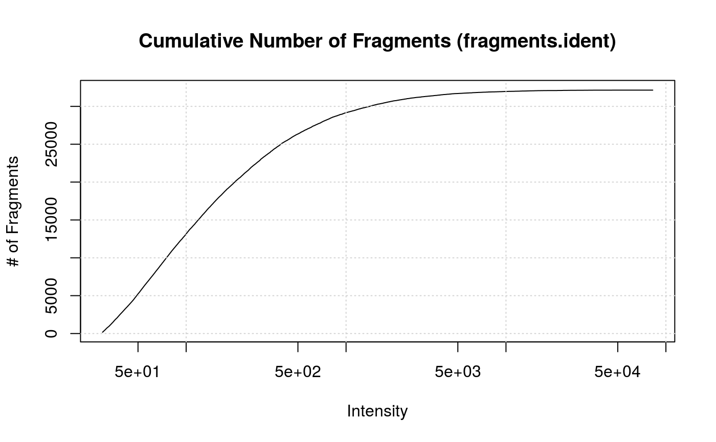

Cumulative Number of Fragments

plotCumulativeNumberOfFragments(synobj2,
                                what = "spectra.quant")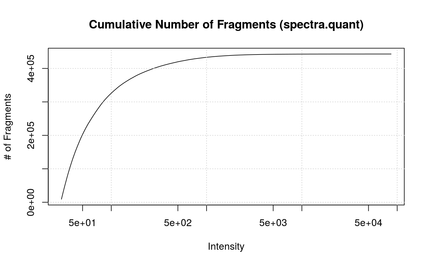

Cumulative Number of Fragments

filterFragments(synobj2,
                what = "fragments.ident",
                minIntensity = 70)
filterFragments(synobj2,
                what = "spectra.quant",
                minIntensity = 70)

Fragment matching

This method, named fragmentMatching, performs the matching of the identification fragments vs the quantitation spectra and counts the number of identical peaks for each combination.

Because the peaks/fragments in the spectra of one run will never be numerically identical to these in another, a tolerance parameter has to be set using the setFragmentMatchingPpmTolerance function. Peaks/Fragments within this tolerance are treated as identical.

setFragmentMatchingPpmTolerance(synobj2, 25)
fragmentMatching(synobj2)

The plotFragmentMatching function illustrates the details of this fragment matching procedure. If it is called without any additional argument every matched pair (fragment vs spectrum) is plotted. One can use the key argument to select a special value in a column (defined by the column argument) of the MatchedEMRTs data.frame. E.g. if one wants to select the fragment matching results with a high number of common peaks, e.g. 28 common peaks:

plotFragmentMatching(synobj2,
                     key = 28,
                     column = "FragmentMatching")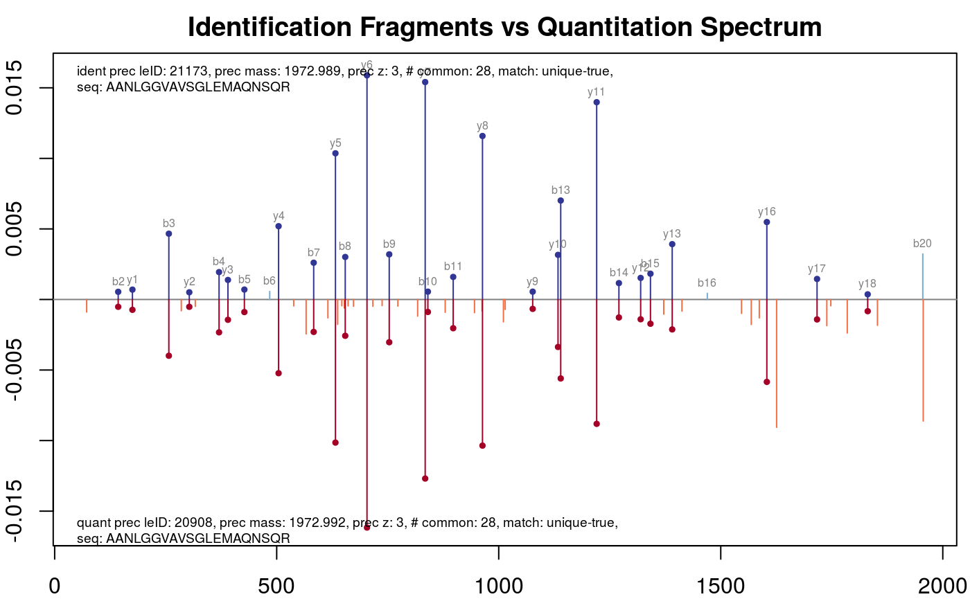

Fragment matching for cases with 28 common fragments. The identification data are shown on the top (blue) and the quantitation data are on the bottom (red). Common peaks are displayed in darker colours and highlighted by full points.

Or, if one is interested in all results for the peptide with the sequence "TALIDGLAQR".

plotFragmentMatching(synobj2,
                     key = "TALIDGLAQR",
                     column = "peptide.seq")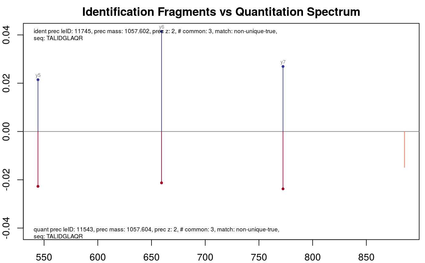

Fragment matching for peptide TALIDGLAQ.

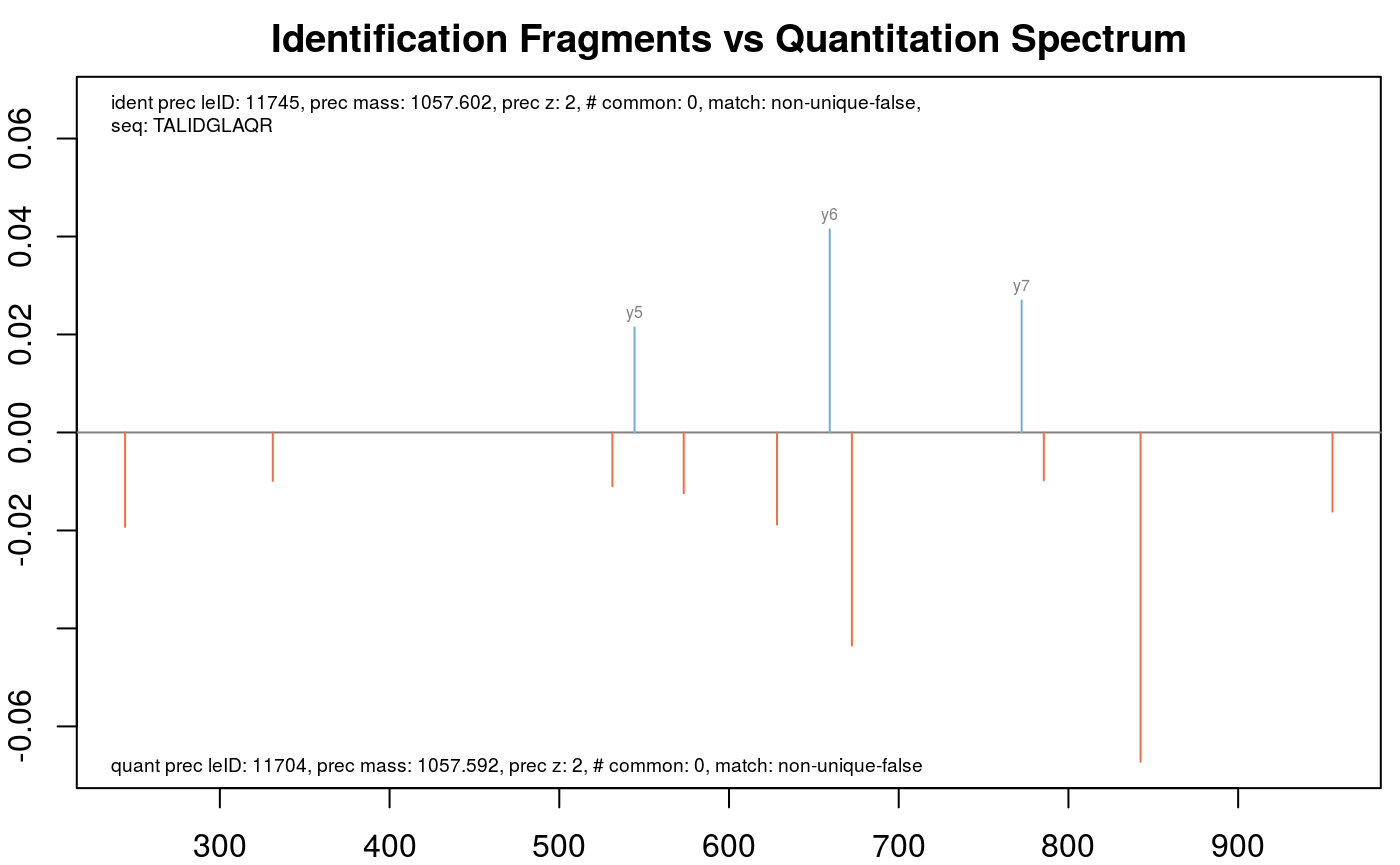
Fragment matching for peptide TALIDGLAQ.

Maybe the peptide with a special precursor ID looks interesting.

plotFragmentMatching(synobj2,
                     key = 12589,
                     column = "precursor.leID.ident")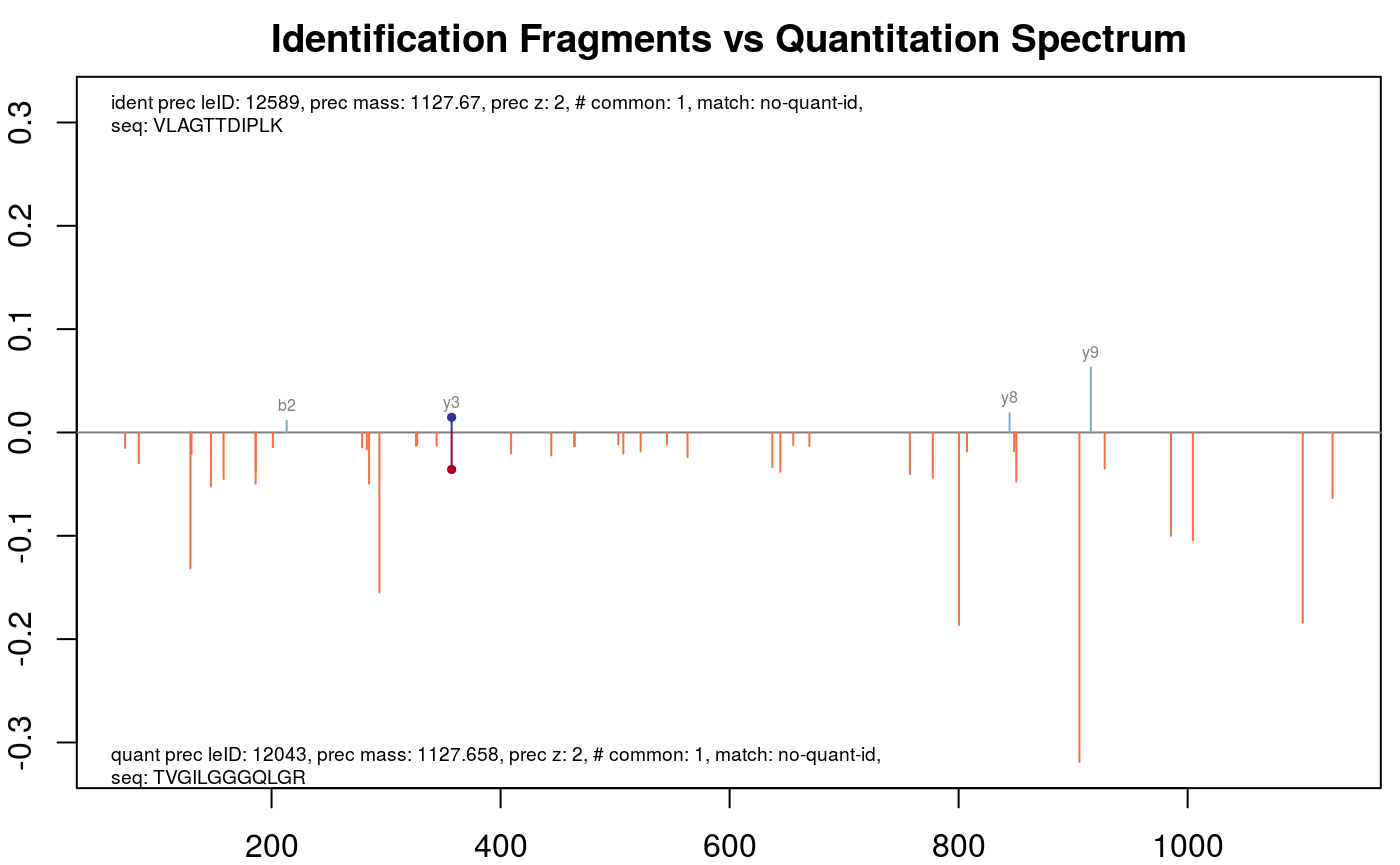

Fragment matching precursor with leID identifier 12589.

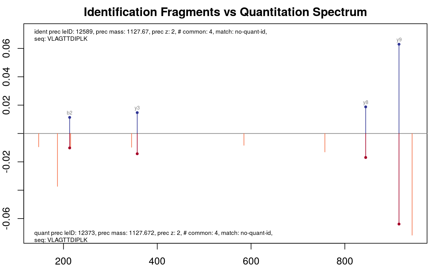
Fragment matching precursor with leID identifier 12589.

Plot distribution of common peaks

The plotFragmentMatchingPerformance function can be used to assess the performance of the fragment matching and the result of the filtering procedure (see below) based on the number of common peaks. This function invisibly returns a list with matrices containing true positive, false positive, true negative and false negative matches for the unique and non unique matches EMRT matches, as illustrated in tables 1 and 2. Both tables could be also generated by fragmentMatchingPerformance.

m <- plotFragmentMatchingPerformance(synobj2)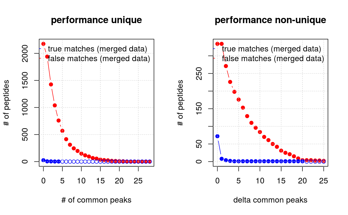

Number of true/false match peptides for different peak matching thresholds and difference in number of peaks between the first and second (in terms of number of common peaks) possible matches. The former metric is used to filter out possible false positive unique matches while the second is used to filter multiple matches. Empty circles indicate zero peptides.

Number of true positives, false negatives, false positives, false negatives and false discovery rate for a given number of common peaks.

ncommon	tp	fp	tn	fn	all	fdr
0	2176	26	0	0	4034	0.0118074
1	1940	5	21	236	2765	0.0025707
2	1426	4	22	750	1899	0.0027972
3	1039	2	24	1137	1370	0.0019212
4	759	2	24	1417	1016	0.0026281
5	569	0	26	1607	780	0.0000000
6	414	0	26	1762	600	0.0000000
7	312	0	26	1864	468	0.0000000
8	245	0	26	1931	379	0.0000000
9	197	0	26	1979	316	0.0000000
10	148	0	26	2028	252	0.0000000
11	116	0	26	2060	203	0.0000000
12	94	0	26	2082	171	0.0000000
13	66	0	26	2110	132	0.0000000
14	55	0	26	2121	110	0.0000000

Number of true positives, false negatives, false positives, false negatives and false discovery rate for a given difference in number of common peaks between the higest and second highest multiply matching EMRTs in terms of number of common peptides.

deltacommon	tp	fp	tn	fn	all	fdr
0	334	72	0	0	4034	0.1773399
1	334	8	64	0	889	0.0233918
2	271	4	68	63	698	0.0145455
3	226	2	70	108	566	0.0087719
4	198	1	71	136	501	0.0050251
5	176	1	71	158	453	0.0056497
6	153	1	71	181	397	0.0064935
7	129	1	71	205	337	0.0076923
8	110	1	71	224	294	0.0090090
9	96	1	71	238	261	0.0103093
10	84	1	71	250	232	0.0117647
11	70	1	71	264	201	0.0140845
12	61	1	71	273	180	0.0161290
13	50	1	71	284	150	0.0196078
14	42	1	71	292	130	0.0232558

Filtering unique matches

From the left panel on figure 7 and table 1 displaying counts for unique matches one can define filtering values for the unique (this section) and multiple matches (next section). In the case of uniquely matching EMRTs, one can easily reduce the number of false matches by requiring that true matches must have at least one peak/fragment in common. Clearly this will also remove some true matches. The question is whether you want to rely on matches that have no (or only a few) peaks/fragments in common?

performance(synobj2)
getEMRTtable(synobj2)

## 
##    0    1    2    3    4    5    6    7   12   14 
##  241 2865  400   64   21    6    5    1    1    1

filterUniqueMatches(synobj2, minNumber = 1)
performance(synobj2)
getEMRTtable(synobj2)

## 
##   -1    0    1    2    3    4    5    6    7   12   14 
##  625  241 2240  400   64   21    6    5    1    1    1

Filtering non-unique matches

The largest benefit of fragment matching is for non unique matches. If we assume that true match have a highest number of common peaks/fragments, we can distinguish correct matches among multiple possible matches that could not resolved before (c.f. section [#sec:plotperf]). To do so, we use the difference of common peaks from the highest to the second highest number in the match group. Assuming two cases with multiple matches. In the first case, we have two possible matches: a match with 7 and a match with 2 fragments in common. In the second ambiguous match, there are a matches with 2 and 1 fragments in common respectively. If we decide to accept a difference of at least 2, our first multiple match case be resolved into a unique match as the difference between the best and second matches is 5 and the best match with 7 common fragments will be upgraded to a unique match.

The right panel of figure 7 and table 2 can be used to choose a good threshold for the difference in number of common peaks.

performance(synobj2)
getEMRTtable(synobj2)

## 
##   -1    0    1    2    3    4    5    6    7   12   14 
##  625  241 2240  400   64   21    6    5    1    1    1

filterNonUniqueMatches(synobj2, minDelta = 2)
performance(synobj2)
getEMRTtable(synobj2)

## 
##   -2   -1    0    1 
##  210  625  241 2529

In this example we rescued 289 unique matches out of the non unique ones.

Exporting results

Like in the initial synapter workflow, it is possible to export the MatchedEMRT results using the writeMatchedEMRTs function. The table has some new columns that correspond to the fragment matching procedure, e.g. FragmentMatching, .

writeMatchedEMRTs(synobj2, file = "MatchedEMRTs.csv")

Session information

All software and respective versions used to produce this document are listed below.

sessionInfo()

## R version 3.5.1 Patched (2018-08-16 r75161)
## Platform: x86_64-pc-linux-gnu (64-bit)
## Running under: Ubuntu 14.04.5 LTS
## 
## Matrix products: default
## BLAS: /usr/lib/atlas-base/atlas/libblas.so.3.0
## LAPACK: /usr/lib/lapack/liblapack.so.3.0
## 
## locale:
##  [1] LC_CTYPE=en_GB.UTF-8       LC_NUMERIC=C              
##  [3] LC_TIME=en_GB.UTF-8        LC_COLLATE=en_GB.UTF-8    
##  [5] LC_MONETARY=en_GB.UTF-8    LC_MESSAGES=en_GB.UTF-8   
##  [7] LC_PAPER=en_GB.UTF-8       LC_NAME=C                 
##  [9] LC_ADDRESS=C               LC_TELEPHONE=C            
## [11] LC_MEASUREMENT=en_GB.UTF-8 LC_IDENTIFICATION=C       
## 
## attached base packages:
## [1] parallel  stats     graphics  grDevices utils     datasets  methods  
## [8] base     
## 
## other attached packages:
##  [1] synapterdata_1.18.0 synapter_2.5.2      MSnbase_2.7.4      
##  [4] ProtGenerics_1.12.0 BiocParallel_1.14.2 mzR_2.15.2         
##  [7] Rcpp_0.12.18        Biobase_2.40.0      BiocGenerics_0.26.0
## [10] BiocStyle_2.8.2    
## 
## loaded via a namespace (and not attached):
##  [1] vsn_3.48.1            splines_3.5.1         foreach_1.4.4        
##  [4] assertthat_0.2.0      highr_0.7             affy_1.58.0          
##  [7] stats4_3.5.1          yaml_2.2.0            impute_1.54.0        
## [10] pillar_1.3.0          backports_1.1.2       lattice_0.20-35      
## [13] glue_1.3.0            limma_3.36.3          digest_0.6.16        
## [16] RColorBrewer_1.1-2    XVector_0.20.0        qvalue_2.12.0        
## [19] colorspace_1.3-2      htmltools_0.3.6       preprocessCore_1.42.0
## [22] Matrix_1.2-14         plyr_1.8.4            MALDIquant_1.18      
## [25] XML_3.98-1.16         pkgconfig_2.0.2       bookdown_0.7         
## [28] zlibbioc_1.26.0       purrr_0.2.5           scales_1.0.0         
## [31] affyio_1.50.0         cleaver_1.18.0        tibble_1.4.2         
## [34] IRanges_2.14.11       ggplot2_3.0.0         lazyeval_0.2.1       
## [37] survival_2.42-6       magrittr_1.5          crayon_1.3.4         
## [40] memoise_1.1.0         evaluate_0.11         fs_1.2.6             
## [43] doParallel_1.0.11     MASS_7.3-50           xml2_1.2.0           
## [46] BiocInstaller_1.30.0  tools_3.5.1           hms_0.4.2            
## [49] stringr_1.3.1         S4Vectors_0.18.3      munsell_0.5.0        
## [52] bindrcpp_0.2.2        Biostrings_2.48.0     pcaMethods_1.72.0    
## [55] compiler_3.5.1        pkgdown_1.1.0         mzID_1.18.0          
## [58] rlang_0.2.2           grid_3.5.1            iterators_1.0.10     
## [61] rmarkdown_1.10        gtable_0.2.0          codetools_0.2-15     
## [64] multtest_2.36.0       roxygen2_6.1.0        reshape2_1.4.3       
## [67] R6_2.2.2              knitr_1.20            dplyr_0.7.6          
## [70] bindr_0.1.1           commonmark_1.5        rprojroot_1.3-2      
## [73] readr_1.1.1           desc_1.2.0            stringi_1.2.4        
## [76] tidyselect_0.2.4      xfun_0.3

References

Bond, Nicholas James, Pavel Vyacheslavovich Shliaha, Kathryn S. Lilley, and Laurent Gatto. 2013. “Improving Qualitative and Quantitative Performance for Ms\(^E\)-Based Label Free Proteomics.” Journal of Proteome Research 12 (6). doi:10.1021/pr300776t.