Abstract

This vignette describes the new functionality implemented version 2.0 of the ‘synapter’ package. It describes the typical workflow including the 3D grid search, fragment matching and correction of detector saturation.

Foreword

synapter is free and open-source software. If you use it, please support the project by citing it in publications:

Nicholas James Bond, Pavel Vyacheslavovich Shliaha, Kathryn S. Lilley, and Laurent Gatto. Improving qualitative and quantitative performance for MS\(^E\)-based label free proteomics. J. Proteome Res., 2013, 12 (6), pp 2340–2353

Questions and bugs

For bugs, typos, suggestions or other questions, please file an issue in our tracking system (https://github.com/lgatto/synapter/issues) providing as much information as possible, a reproducible example and the output of sessionInfo().

If you don’t have a GitHub account or wish to reach a broader audience for general questions about proteomics analysis using R, you may want to use the Bioconductor support site: https://support.bioconductor.org/.

Introduction

Here we describe the new functionality implemented in synapter 2.0. Namely this vignette covers the utilisation of the new 3D grid search, the fragment matching, intensity modeling and correction of detector saturation.

Workflow

The synapter2 workflow is similar to the old one in synapter1. First it is necessary to use PLGS to create the csv (and xml) files. Therefore we refer the reader to the default synapter vignette, available online and with vignette("synapter", package = "synapter").

In contrast to the original workflow the final_fragment.csv file for the identification run and a Spectrum.xml file for the quantification run are needed if the fragment matching should be applied.

Subsequently the original workflow is enhanced by the new 3D grid search and the intensity modeling. Afterwards the fragment matching could be applied. MSnbase (Gatto and Lilley 2012) is used for further analysis. The new synapter adds synapter/PLGS consensus filtering and the detector saturation correction for MSnSets.

New synapter workflow. Dark green boxes show the traditional synapter1 part and the light green boxes highlight the new synapter2 functionality.

Step-by-step workflow

Create a `Synapter` object

To demonstrate a typical step-by-step workflow we use example data that are available on http://proteome.sysbiol.cam.ac.uk/lgatto/synapter/data/. There is also an synobj2 object in synapterdata which contains the same data.

The Synapter constructor uses a named list of input files. Please note that we add identfragments (final_fragment.csv) and quantspectra (Spectrum.xml) because we want to apply the fragment matching later.

## Please find the raw data at:
## http://proteome.sysbiol.cam.ac.uk/lgatto/synapter/data/
library("synapter")

inlist <- list(
  identpeptide = "fermentor_03_sample_01_HDMSE_01_IA_final_peptide.csv.gz",
  identfragments = "fermentor_03_sample_01_HDMSE_01_IA_final_fragment.csv.gz",
  quantpeptide = "fermentor_02_sample_01_HDMSE_01_IA_final_peptide.csv.gz",
  quantpep3d = "fermentor_02_sample_01_HDMSE_01_Pep3DAMRT.csv.gz",
  quantspectra = "fermentor_02_sample_01_HDMSE_01_Pep3D_Spectrum.xml.gz",
  fasta = "S.cerevisiae_Uniprot_reference_canonical_18_03_14.fasta")

synobj2 <- Synapter(inlist, master=FALSE)

synobj2

## Object of class "Synapter" 
## Class version 2.0.0 
## Package version 1.99.0 
## Data files:
##  + Identification pep file: fermentor_03_sample_01_HDMSE_01_IA_final_peptide.csv.gz 
##  + Identification Fragment file: fermentor_02_sample_01_HDMSE_01_Pep3D_Spectrum.xml.gz 
##  + Quantitation pep file: fermentor_02_sample_01_HDMSE_01_IA_final_peptide.csv.gz 
##  + Quantitation Pep3DAMRT file: fermentor_02_sample_01_HDMSE_01_Pep3DAMRT.csv.gz 
##  + Quantitation Spectrum file: fermentor_02_sample_01_HDMSE_01_Pep3D_Spectrum.xml.gz 
##  + Fasta file: S.cerevisiae_Uniprot_reference_canonical_18_03_14.fasta 
## Log:
## [1] "Instance created on Tue Apr  4 09:01:34 2017"
## [2] "Read identification peptide data [11471,16]" 
## [ 10 lines ]
## [13] "Read identification fragment data [7078]"
## [14] "Read quantitation spectra [36539]"

Filtering

The first steps in each synapter analysis are filtering by peptide sequence, peptide length, ppm error and false positive rate.

Here we use the default values for each method. But the accompanying plotting methods should be used to find the best threshold:

filterUniqueDbPeptides(synobj2,
                       missedCleavages=0,
                       IisL=TRUE)
filterPeptideLength(synobj2, l=7)
plotFdr(synobj2)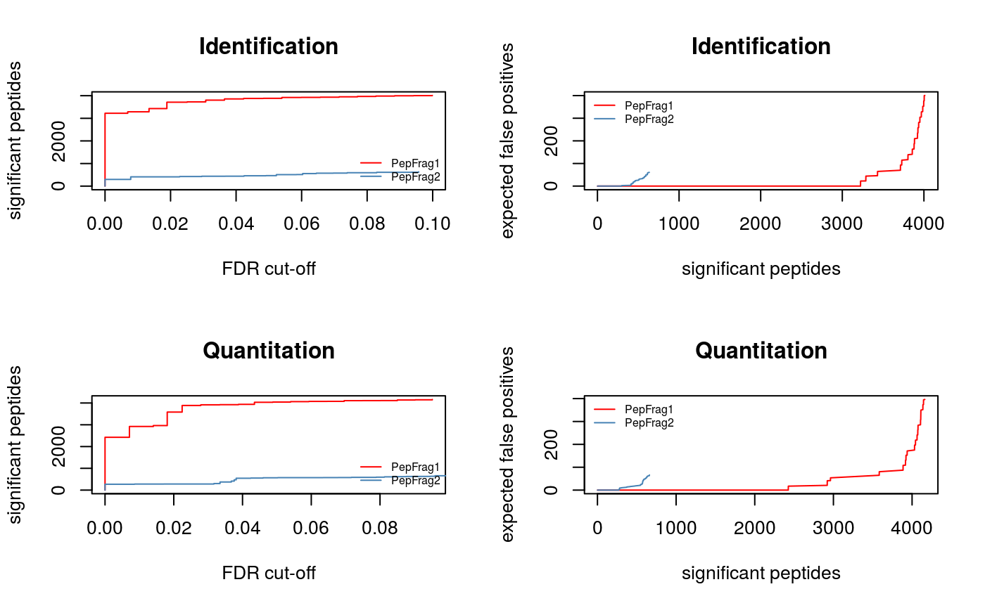

filterQuantPepScore(synobj2, method="BH",
                    fdr=0.05)
filterIdentPepScore(synobj2, method="BH",
                    fdr=0.05)
par(mfcol=c(1, 2))
plotPpmError(synobj2, what="Ident")
plotPpmError(synobj2, what="Quant")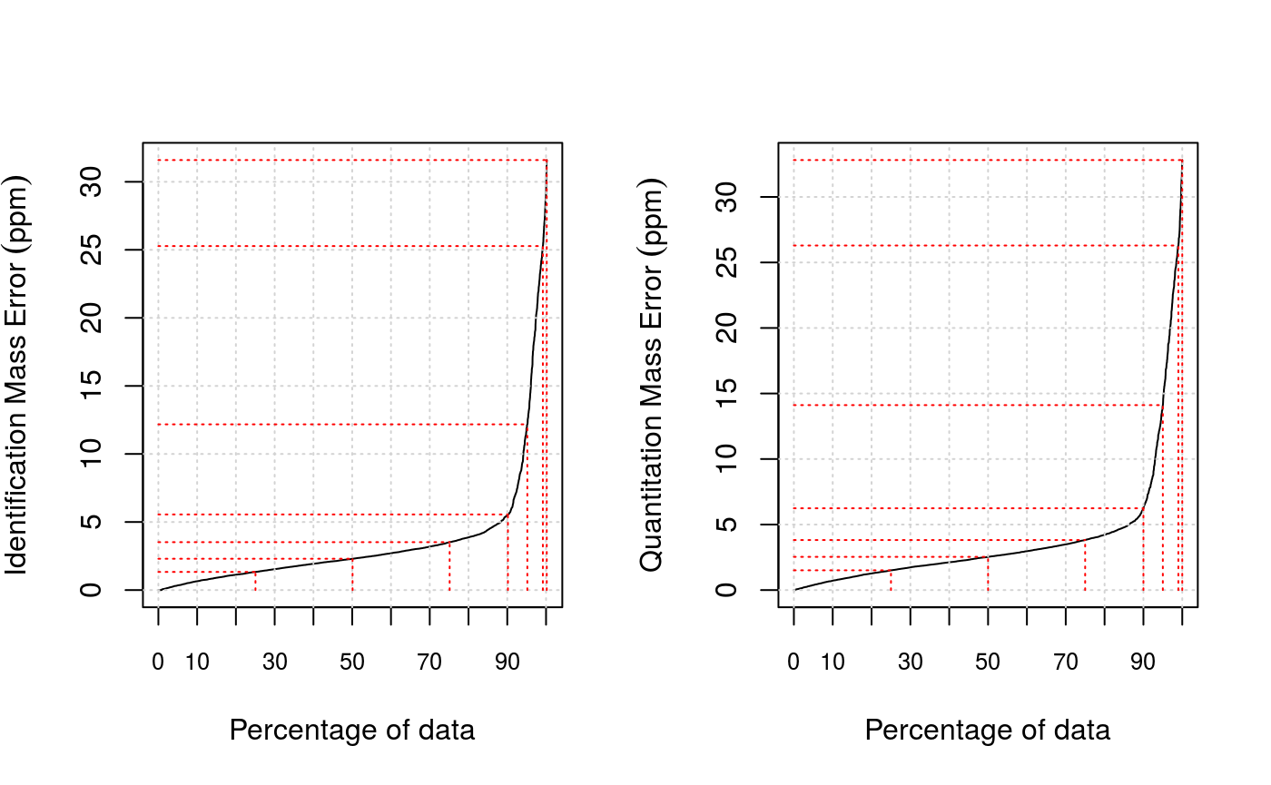

par(mfcol=c(1, 1))
filterQuantPpmError(synobj2, ppm=20)
filterIdentPpmError(synobj2, ppm=20)
plotPepScores(synobj2)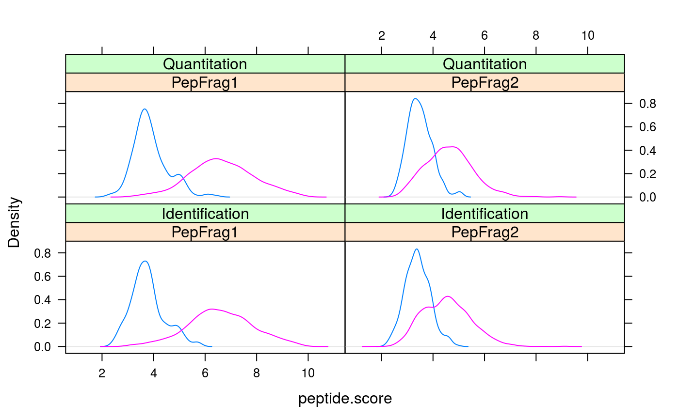

filterIdentProtFpr(synobj2, fpr=0.05)
filterQuantProtFpr(synobj2, fpr=0.05)

Modeling retention time

Next we merge the identified peptides from the identification run and quantification run and build a LOWESS based retention time model to remove systematic shifts in the retention times. Here we use the default values but as stated above the plotting methods should be used to find sensible thresholds.

mergePeptides(synobj2)

plotRt(synobj2, what="data")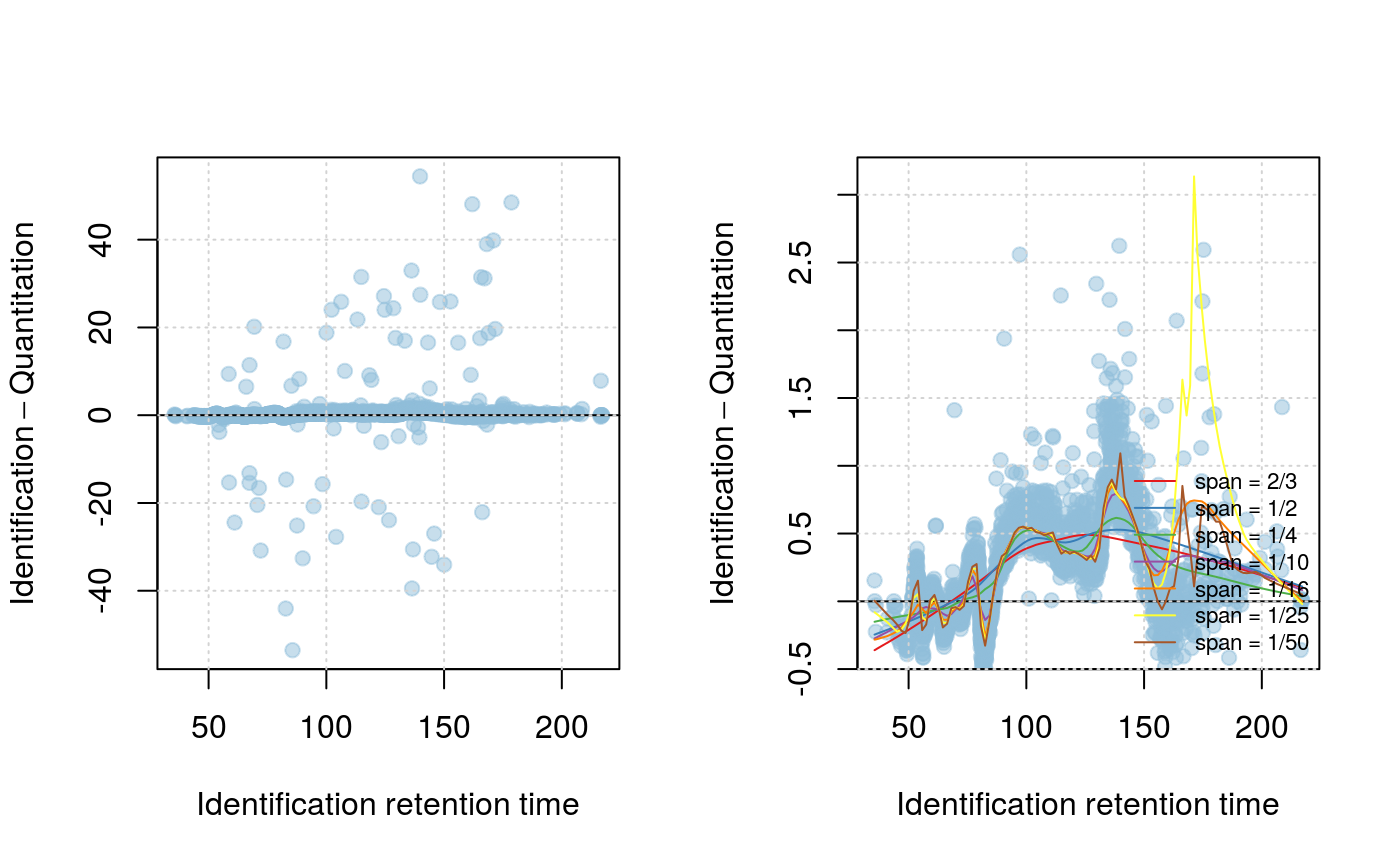

setLowessSpan(synobj2, span=0.05)
modelRt(synobj2)

par(mfcol=c(1, 2))
plotRtDiffs(synobj2)
plotRt(synobj2, what="model", nsd=1)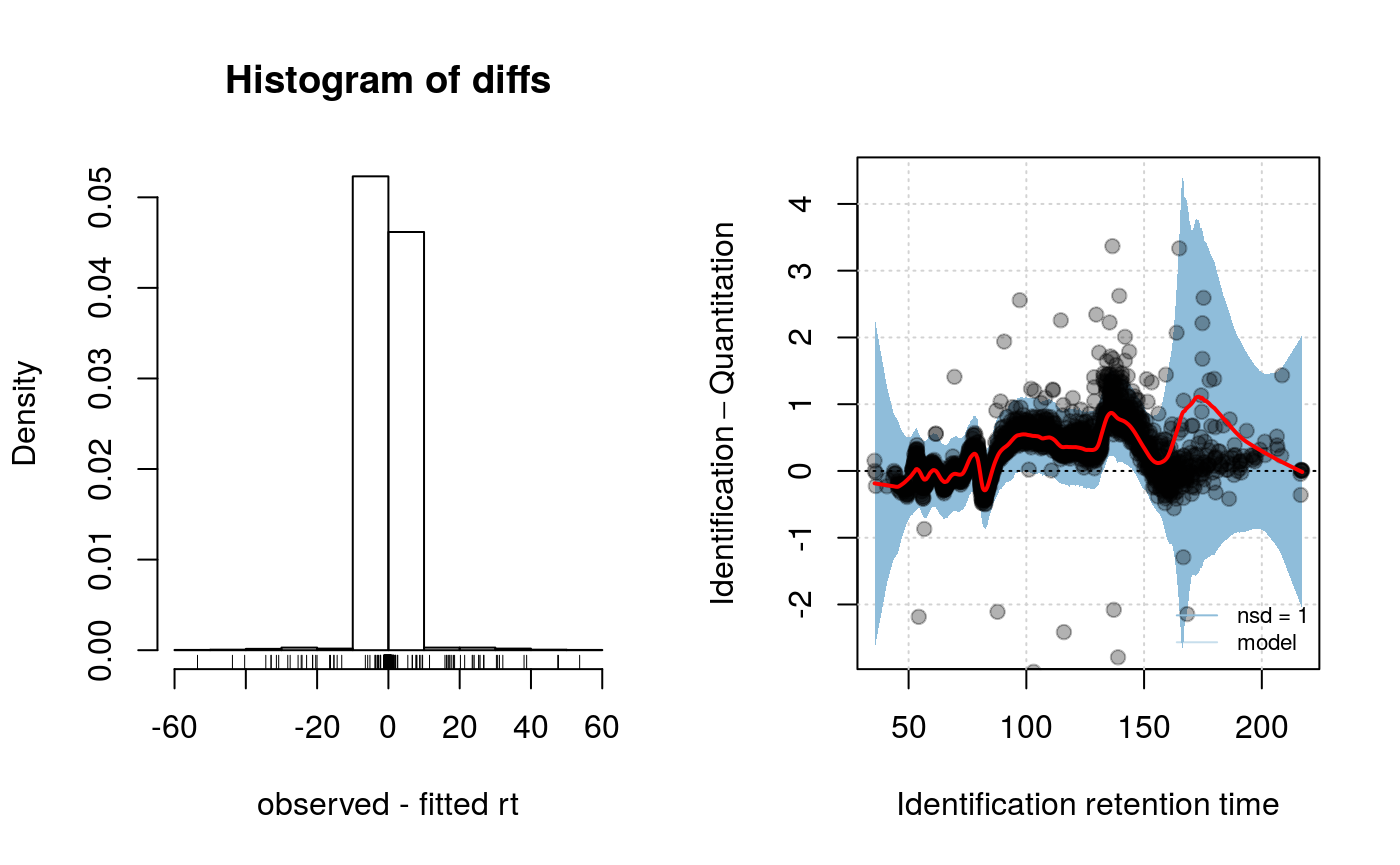

par(mfcol=c(1, 1))

plotFeatures(synobj2, what="all", ionmobility=TRUE)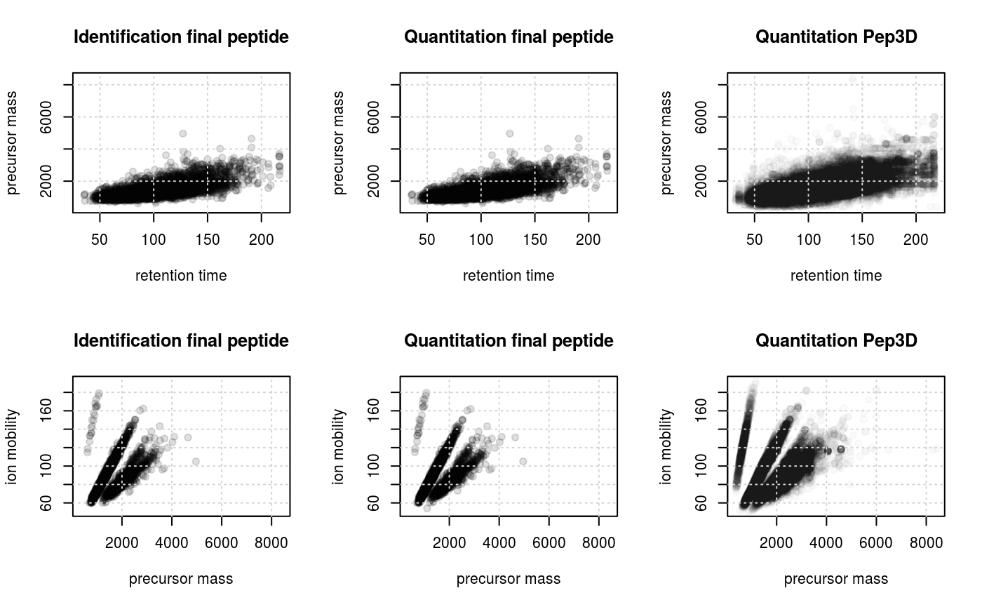

Grid search

To find EMRTS (exact m/z-retention time pairs) we try are running a grid search to find the best retention time tolerance and m/z tolerance that results in the most correct one-to-one matching in the merged (already identified) data. If the identification and quantitation run are HDMS\(^E\) data we could use the new 3D grid search that looks for the best matching in the retention time, m/z and ion mobility (drift time) domain to increase the accuracy. If one or both datasets are MS\(^E\) data it falls back to the traditional 2D grid search.

searchGrid(synobj2,
           imdiffs=seq(from=0.6, to=1.6, by=0.2),
           ppms=seq(from=2, to=20, by=2),
           nsds=seq(from=0.5, to=5, by=0.5))
setBestGridParams(synobj2)
findEMRTs(synobj2)
plotEMRTtable(synobj2)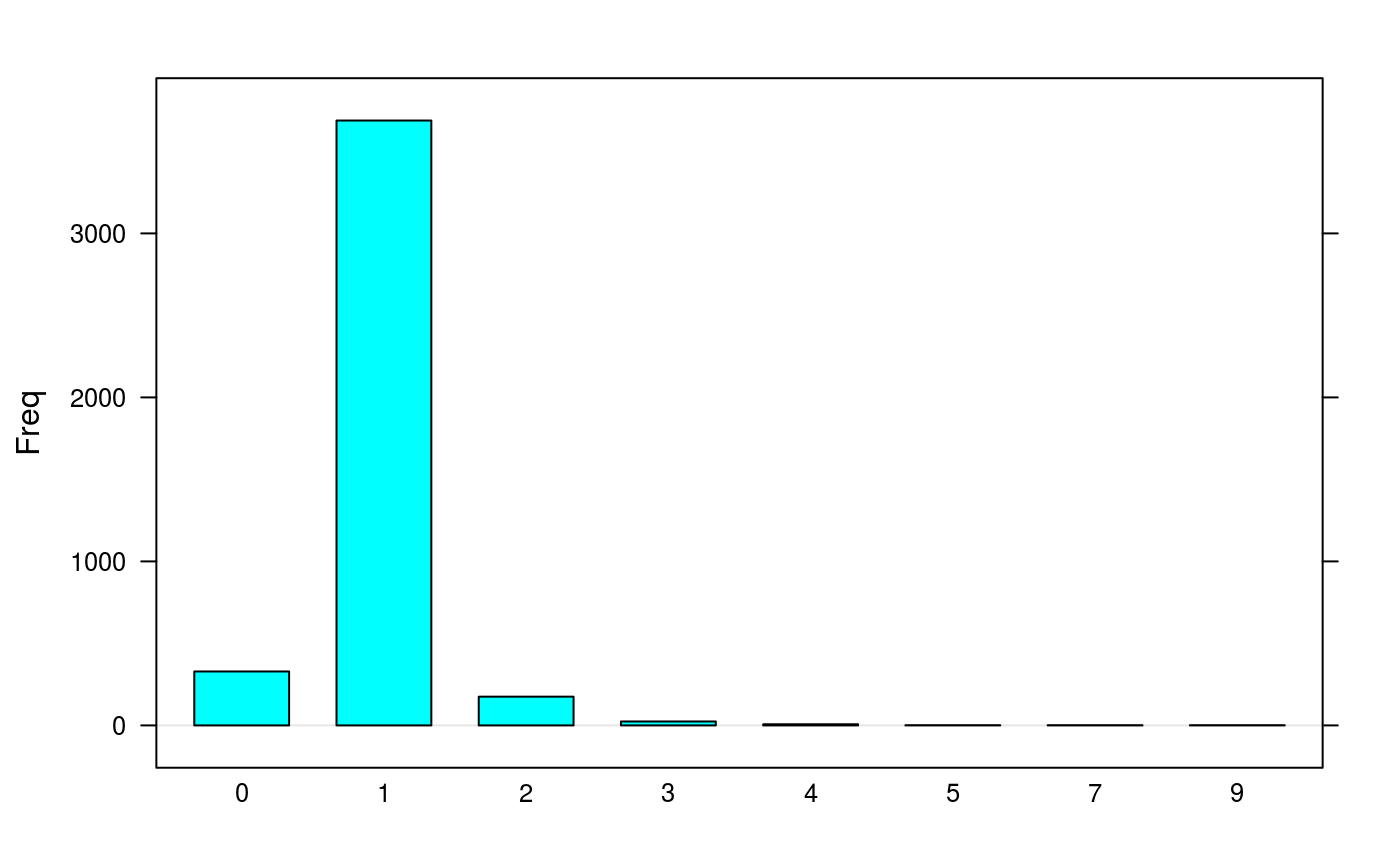

Fragment matching

For the details of the fragment matching procedure we refer to the fragment matching vignette that is available online and with vignette("fragmentmatching", package = "synapter"). Briefly we compare the fragments of the identification run with the spectra from the quantification run and remove entries where there are very few/none common peaks/fragments between them.

First we starting by removing less intense fragments and peaks.

filterFragments(synobj2,
                what="fragments.ident",
                minIntensity=70)
filterFragments(synobj2,
                what="spectra.quant",
                minIntensity=70)

Next we look for common peaks via fragmentMatching:

fragmentMatching(synobj2)

## Warning in object$fragmentMatching(verbose = verbose): FragmentMatching ppm
## tolerance undefined. Setting to default value.

We get tables for unique and non-unique matches:

knitr::kable(fragmentMatchingPerformance(synobj2,
                                         what="unique"))

ncommon	tp	fp	tn	fn	all	fdr
0	3097	79	0	0	4159	0.0248741
1	2556	22	57	541	2864	0.0085337
2	1682	12	67	1415	1864	0.0070838
3	1193	4	75	1904	1339	0.0033417
4	862	1	78	2235	987	0.0011587
5	651	1	78	2446	754	0.0015337
6	488	1	78	2609	578	0.0020450
7	372	1	78	2725	453	0.0026810
8	294	0	79	2803	367	0.0000000
9	240	0	79	2857	307	0.0000000
10	186	0	79	2911	245	0.0000000
11	149	0	79	2948	197	0.0000000
12	124	0	79	2973	165	0.0000000
13	95	0	79	3002	126	0.0000000
14	82	0	79	3015	105	0.0000000
15	59	0	79	3038	76	0.0000000
16	48	0	79	3049	61	0.0000000
17	41	0	79	3056	53	0.0000000
18	27	0	79	3070	36	0.0000000
19	21	0	79	3076	26	0.0000000
20	14	0	79	3083	16	0.0000000
21	12	0	79	3085	14	0.0000000
22	8	0	79	3089	10	0.0000000
23	6	0	79	3091	8	0.0000000
24	5	0	79	3092	6	0.0000000
25	4	0	79	3093	5	0.0000000
26	3	0	79	3094	3	0.0000000
27	3	0	79	3094	3	0.0000000
28	1	0	79	3096	1	0.0000000

knitr::kable(fragmentMatchingPerformance(synobj2,
                                         what="non-unique"))

deltacommon	tp	fp	tn	fn	all	fdr
0	163	33	0	0	4159	0.1683673
1	163	2	31	0	374	0.0121212
2	132	1	32	31	304	0.0075188
3	119	1	32	44	276	0.0083333
4	110	0	33	53	256	0.0000000
5	95	0	33	68	226	0.0000000
6	85	0	33	78	202	0.0000000
7	75	0	33	88	178	0.0000000
8	67	0	33	96	161	0.0000000
9	60	0	33	103	145	0.0000000
10	53	0	33	110	127	0.0000000
11	43	0	33	120	106	0.0000000
12	37	0	33	126	92	0.0000000
13	27	0	33	136	71	0.0000000
14	20	0	33	143	56	0.0000000
15	12	0	33	151	37	0.0000000
16	10	0	33	153	26	0.0000000
17	8	0	33	155	21	0.0000000
18	7	0	33	156	18	0.0000000
19	4	0	33	159	9	0.0000000
20	2	0	33	161	5	0.0000000
21	2	0	33	161	5	0.0000000
22	2	0	33	161	5	0.0000000
23	1	0	33	162	3	0.0000000
24	1	0	33	162	3	0.0000000
25	1	0	33	162	3	0.0000000

Subsequently we could filter by minimal accepted common peaks:

filterUniqueMatches(synobj2, minNumber=1)
filterNonUniqueMatches(synobj2, minDelta=2)
filterNonUniqueIdentMatches(synobj2)

Finally we rescue EMRTs that are filtered but were identified by PLGS:

rescueEMRTs(synobj2, method="rescue")

Modeling intensity

In a similar manner as correcting for the retention time drift we correct systematic errors of the intensity via a LOWESS model. The function modelIntensity has to applied after findEMRTs. The model is build on the merged peptides as it is done for the retention time model. But in contrast to the retention time model the prediction is necessary for the matched quantitation data.

plotIntensity(synobj2, what="data")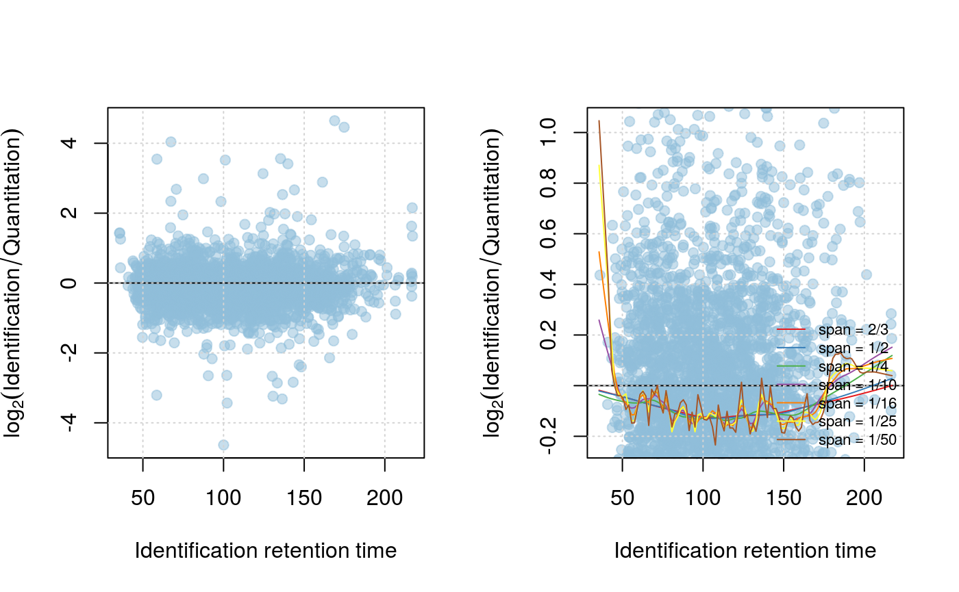

setLowessSpan(synobj2, 0.05)
modelIntensity(synobj2)
plotIntensity(synobj2, what="model", nsd=1)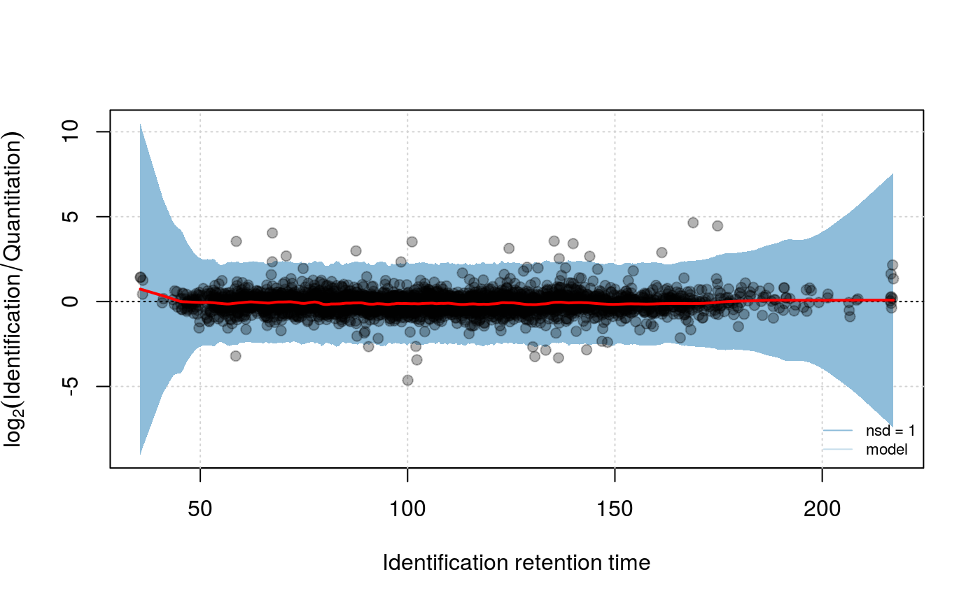

`synergise2`

The whole workflow described in the step-by-step workflow is wrapped in the synergise2 function. As side effect it generates a nice HTML report. An example could be found on https://github.com/lgatto/synapter.

synobj2 <- synergise2(filenames = inlist,
                      outputdir = ".")

synapter/PLGS agreement

For the next steps we need to convert the Synapter object into an MSnSet.

msn <- as(synobj2, "MSnSet")

Subsequently we look for synapter/PLGS agreement (this is more useful for a combined MSnSet; see basic synapter online or with vignette("synapter", package = "synapter")). synapterPlgsAgreement adds an agreement column for each sample and counts the agreement/disagreement in additional columns:

msn <- synapterPlgsAgreement(msn)
knitr::kable(head(fData(msn)[, grepl("[Aa]gree",
                                     fvarLabels(msn)),
                             drop=FALSE]))

	synapterPlgsAgreement.fermentor_02_sample_01_HDMSE_01	nAgree	synapterPlgsAgreementRatio
NVNDVIAPAFVK	agree	1	1
TAGIQIVADDLTVTNPK	agree	1	1
WLTGPQLADLYHSLMK	agree	1	1
AAQDSFAAGWGVMVSHR	agree	1	1
TFAEALR	agree	1	1
LGANAILGVSLAASR	no_synapter_transfer	0	NaN

Correction of detector saturation

As described in (Shliaha et al. 2013) Synapt G2 devices suffer from detector saturation. This could be partly corrected by requantify. Therefore a saturationThreshold has to be given above that intensity saturation potentially happens. There are several methods available.

msncor <- requantify(msn,
                     saturationThreshold=1e5,
                     method="sum")

If an MSnSet object was requantified using the "sum" requantification method TOP3 normalisation is not valid anymore because the most abundant proteins are penalised by removing high intensity isotopes (for details see ?requantify and ?rescaleForTop3). This could be overcome by calling rescaleForTop3:

msncor <- rescaleForTop3(before=msn,
                         after=msncor,
                         saturationThreshold=1e5)

New functions not covered in this vignette

Since synapter 2.0 makeMaster supports fragment files as well. It is possible to create a fragment library that could used for fragment matching because of the large data this could not covered in this vignette. An introduction how to create a master could be found in the basic synapter vignette, available online or with vignette("synapter", package = "synapter"). Please find details about creating a fragment library in ?makeMaster.

Session information

All software and respective versions used to produce this document are listed below.

sessionInfo()

## R version 3.5.1 Patched (2018-08-16 r75161)
## Platform: x86_64-pc-linux-gnu (64-bit)
## Running under: Ubuntu 14.04.5 LTS
## 
## Matrix products: default
## BLAS: /usr/lib/atlas-base/atlas/libblas.so.3.0
## LAPACK: /usr/lib/lapack/liblapack.so.3.0
## 
## locale:
##  [1] LC_CTYPE=en_GB.UTF-8       LC_NUMERIC=C              
##  [3] LC_TIME=en_GB.UTF-8        LC_COLLATE=en_GB.UTF-8    
##  [5] LC_MONETARY=en_GB.UTF-8    LC_MESSAGES=en_GB.UTF-8   
##  [7] LC_PAPER=en_GB.UTF-8       LC_NAME=C                 
##  [9] LC_ADDRESS=C               LC_TELEPHONE=C            
## [11] LC_MEASUREMENT=en_GB.UTF-8 LC_IDENTIFICATION=C       
## 
## attached base packages:
## [1] parallel  stats     graphics  grDevices utils     datasets  methods  
## [8] base     
## 
## other attached packages:
##  [1] synapterdata_1.18.0 synapter_2.5.2      MSnbase_2.7.4      
##  [4] ProtGenerics_1.12.0 BiocParallel_1.14.2 mzR_2.15.2         
##  [7] Rcpp_0.12.18        Biobase_2.40.0      BiocGenerics_0.26.0
## [10] BiocStyle_2.8.2    
## 
## loaded via a namespace (and not attached):
##  [1] vsn_3.48.1            splines_3.5.1         foreach_1.4.4        
##  [4] assertthat_0.2.0      highr_0.7             affy_1.58.0          
##  [7] stats4_3.5.1          yaml_2.2.0            impute_1.54.0        
## [10] pillar_1.3.0          backports_1.1.2       lattice_0.20-35      
## [13] glue_1.3.0            limma_3.36.3          digest_0.6.16        
## [16] RColorBrewer_1.1-2    XVector_0.20.0        qvalue_2.12.0        
## [19] colorspace_1.3-2      htmltools_0.3.6       preprocessCore_1.42.0
## [22] Matrix_1.2-14         plyr_1.8.4            MALDIquant_1.18      
## [25] XML_3.98-1.16         pkgconfig_2.0.2       bookdown_0.7         
## [28] zlibbioc_1.26.0       purrr_0.2.5           scales_1.0.0         
## [31] affyio_1.50.0         cleaver_1.18.0        tibble_1.4.2         
## [34] IRanges_2.14.11       ggplot2_3.0.0         lazyeval_0.2.1       
## [37] survival_2.42-6       magrittr_1.5          crayon_1.3.4         
## [40] memoise_1.1.0         evaluate_0.11         fs_1.2.6             
## [43] doParallel_1.0.11     MASS_7.3-50           xml2_1.2.0           
## [46] BiocInstaller_1.30.0  tools_3.5.1           hms_0.4.2            
## [49] stringr_1.3.1         S4Vectors_0.18.3      munsell_0.5.0        
## [52] bindrcpp_0.2.2        Biostrings_2.48.0     pcaMethods_1.72.0    
## [55] compiler_3.5.1        pkgdown_1.1.0         mzID_1.18.0          
## [58] rlang_0.2.2           grid_3.5.1            iterators_1.0.10     
## [61] rmarkdown_1.10        gtable_0.2.0          codetools_0.2-15     
## [64] multtest_2.36.0       roxygen2_6.1.0        reshape2_1.4.3       
## [67] R6_2.2.2              knitr_1.20            dplyr_0.7.6          
## [70] bindr_0.1.1           commonmark_1.5        rprojroot_1.3-2      
## [73] readr_1.1.1           desc_1.2.0            stringi_1.2.4        
## [76] tidyselect_0.2.4      xfun_0.3

References

Gatto, Laurent, and Kathryn S Lilley. 2012. “MSnbase – an R/Bioconductor Package for Isobaric Tagged Mass Spectrometry Data Visualization, Processing and Quantitation.” Bioinformatics 28 (2): 288–9. doi:10.1093/bioinformatics/btr645.

Shliaha, Pavel Vyacheslavovich, Nicholas James Bond, Laurent Gatto, and Kathryn S. Lilley. 2013. “The Effects of Travelling Wave Ion Mobility Separation on Data Independent Acquisition in Proteomics Studies.” Journal of Proteome Research 2 (6). doi:10.1021/pr300775k.

Synapter2 and synergise2

Laurent Gatto

Sebastian Gibb

Pavel V. Shliaha

Foreword

Questions and bugs

Introduction

Workflow

Step-by-step workflow

Create a `Synapter` object

Filtering

Modeling retention time

Grid search

Fragment matching

Modeling intensity

`synergise2`

synapter/PLGS agreement

Correction of detector saturation

New functions not covered in this vignette

Session information

References

Contents

Synapter2 and synergise2

Laurent Gatto

Sebastian Gibb

Pavel V. Shliaha

Foreword

Questions and bugs

Introduction

Workflow

Step-by-step workflow

Create a Synapter object

Filtering

Modeling retention time

Grid search

Fragment matching

Modeling intensity

synergise2

synapter/PLGS agreement

Correction of detector saturation

New functions not covered in this vignette

Session information

References

Contents

Create a `Synapter` object

`synergise2`