
New feature: annotated chromatograms
Today, I’m going to introduce a recent feature from the Spectra package, namely annotated chromatograms. I’ll start by showing the result and them explain how to produce it.
An annotated chromatogram
You will immediately recognise a chromatogram on the figure below, showing MS1 scan total ion current over the experiment’s retention time. Each MS1 event is highlighted by a dot which is colour-coded based on the number of MS2 offspring scans that lead to identifications. Grey dots are MS1 scans without any identified precursor peaks while coloured dots (from dark to light blue) represent MS1 scans have 1 to 10 (in one case, see details below) identified precursor peaks.

You can also watch a video illustrating this post here.
The data
The generate the data for an annotated chromatogram, we need raw and identification data and join them together. We will use the TMT_Erwinia data available in the msdata. Below, we get the raw and identification data files.
library("msdata")
basename(mzml_file <- proteomics(pattern = "20141210.mzML", full.names = TRUE))
## [1] "TMT_Erwinia_1uLSike_Top10HCD_isol2_45stepped_60min_01-20141210.mzML.gz"basename(mzid_file <- ident(pattern = "20141210.mzid", full.names = TRUE))## [1] "TMT_Erwinia_1uLSike_Top10HCD_isol2_45stepped_60min_01-20141210.mzid"Here, we load the raw data into R as a Spectra object:
library("Spectra")
rw <- Spectra(mzml_file)
rw
## MSn data (Spectra) with 7534 spectra in a MsBackendMzR backend:
## msLevel rtime scanIndex
## <integer> <numeric> <integer>
## 1 1 0.4584 1
## 2 1 0.9725 2
## 3 1 1.8524 3
## 4 1 2.7424 4
## 5 1 3.6124 5
## ... ... ... ...
## 7530 2 3600.47 7530
## 7531 2 3600.83 7531
## 7532 2 3601.18 7532
## 7533 2 3601.57 7533
## 7534 2 3601.98 7534
## ... 33 more variables/columns.
##
## file(s):
## TMT_Erwinia_1uLSike_Top10HCD_isol2_45stepped_60min_01-20141210.mzML.gzBelow, we load the identification data into R as a PSM object and
filter the PSMs:
library("PSMatch")
id <- PSM(mzid_file) |>
   filterPSMs()
id
## PSM with 2666 rows and 35 columns.
## Spectra: 2646 unique
## db: 2666 target, 0 decoy
## ranks: 1:2666
## Peptides: 2324 unique, 0 multiple
## Proteins: 1466
## names(35): sequence spectrumID ... subReplacementResidue subLocationWe can now annotate the spectra with the identification data. For details about these steps, see the details and example of the joinSpectraData() function.
rw <- joinSpectraData(rw, id,
                by.x = "spectrumId",
                by.y = "spectrumID")
head(na.omit(rw$sequence))
## [1] "ERKLIKKIAKTLVK" "IVILVLIVLFIQKR" "THSQEEMQHMQR" "IDHRSIRVQYK"
## [5] "THSQEEMQHMQR" "RNYKTNNLYLKLK"The countIdentifications() function
The function that permit to produce the data for the figure above is countIdentifications().
The function is going to tally the number of identifications (i.e
non-missing characters in the sequence spectra variable) for each
scan. In the case of MS2 scans, these will be either 1 or 0, depending
the presence of a sequence. For MS1 scans, the function will count the
number of sequences for the descendant MS2 scans, i.e. those produced
from precursor ions from each MS1 scan.
rw <- countIdentifications(rw)Below, we see on the second line that 3457 MS2 scans lead to no PSM, while 2546 lead to an identification. Among all MS1 scans, 833 lead to no MS2 scans with PSMs. 30 MS1 scans generated one MS2 scan that lead to a PSM, 45 lead to two PSMs, …
table(msLevel(rw), rw$countIdentifications)##
## 0 1 2 3 4 5 6 7 8 9 10
## 1 833 30 45 97 139 132 92 42 17 3 1
## 2 3457 2646 0 0 0 0 0 0 0 0 0We can now use this new countIdentifications variable to generate
our annotated chromatogram. The code chunk below filters MS1 level
data and then extracts the spectra variable, in particular the
retention time rtime, the total ion current totIonCurrent and the
newly created countIdentifications to produce a figure with
ggplot2.
library(tidyverse)
rw |>
filterMsLevel(1) |>
spectraData() |>
as_tibble() |>
ggplot(aes(x = rtime,
           y = totIonCurrent)) +
    geom_line(alpha = 0.25) +
    geom_point(aes(colour = ifelse(countIdentifications == 0,
                                   NA, countIdentifications)),
               size = 1,
               alpha = 0.5) +
    labs(colour = "Number of ids")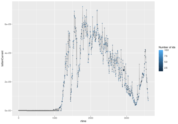
More details and session information
For details about the Spectra package, see the package web
page and the R for
Mass Spectrometry
tutorial.
sessionInfo()## R version 4.1.2 (2021-11-01)
## Platform: x86_64-pc-linux-gnu (64-bit)
## Running under: Ubuntu 20.04.3 LTS
##
## Matrix products: default
## BLAS: /usr/lib/x86_64-linux-gnu/atlas/libblas.so.3.10.3
## LAPACK: /usr/lib/x86_64-linux-gnu/atlas/liblapack.so.3.10.3
##
## locale:
## [1] LC_CTYPE=en_US.UTF-8 LC_NUMERIC=C
## [3] LC_TIME=en_GB.UTF-8 LC_COLLATE=en_US.UTF-8
## [5] LC_MONETARY=en_GB.UTF-8 LC_MESSAGES=en_US.UTF-8
## [7] LC_PAPER=en_GB.UTF-8 LC_NAME=C
## [9] LC_ADDRESS=C LC_TELEPHONE=C
## [11] LC_MEASUREMENT=en_GB.UTF-8 LC_IDENTIFICATION=C
##
## attached base packages:
## [1] stats4 stats graphics grDevices utils datasets methods
## [8] base
##
## other attached packages:
## [1] forcats_0.5.1 stringr_1.4.0 dplyr_1.0.7
## [4] purrr_0.3.4 readr_2.1.1 tidyr_1.1.4
## [7] tibble_3.1.6 ggplot2_3.3.5 tidyverse_1.3.1
## [10] PSMatch_0.7.1 Spectra_1.5.2 ProtGenerics_1.26.0
## [13] BiocParallel_1.28.2 S4Vectors_0.32.3 BiocGenerics_0.40.0
## [16] msdata_0.34.0 knitr_1.36
##
## loaded via a namespace (and not attached):
## [1] bitops_1.0-7 matrixStats_0.61.0
## [3] fs_1.5.1 lubridate_1.8.0
## [5] httr_1.4.2 GenomeInfoDb_1.30.0
## [7] tools_4.1.2 backports_1.4.0
## [9] utf8_1.2.2 R6_2.5.1
## [11] DBI_1.1.1 lazyeval_0.2.2
## [13] colorspace_2.0-2 withr_2.4.3
## [15] tidyselect_1.1.1 compiler_4.1.2
## [17] cli_3.1.0 rvest_1.0.2
## [19] Biobase_2.54.0 xml2_1.3.3
## [21] DelayedArray_0.20.0 labeling_0.4.2
## [23] scales_1.1.1 digest_0.6.29
## [25] XVector_0.34.0 pkgconfig_2.0.3
## [27] MatrixGenerics_1.6.0 highr_0.9
## [29] dbplyr_2.1.1 rlang_0.4.12
## [31] readxl_1.3.1 rstudioapi_0.13
## [33] farver_2.1.0 generics_0.1.1
## [35] jsonlite_1.7.2 RCurl_1.98-1.5
## [37] magrittr_2.0.1 GenomeInfoDbData_1.2.7
## [39] Matrix_1.4-0 Rcpp_1.0.7
## [41] munsell_0.5.0 fansi_0.5.0
## [43] MsCoreUtils_1.6.0 lifecycle_1.0.1
## [45] stringi_1.7.6 MASS_7.3-54
## [47] SummarizedExperiment_1.24.0 zlibbioc_1.40.0
## [49] grid_4.1.2 parallel_4.1.2
## [51] crayon_1.4.2 lattice_0.20-45
## [53] haven_2.4.3 hms_1.1.1
## [55] mzR_2.28.0 pillar_1.6.4
## [57] igraph_1.2.9 GenomicRanges_1.46.1
## [59] QFeatures_1.4.0 codetools_0.2-18
## [61] reprex_2.0.1 glue_1.5.1
## [63] evaluate_0.14 modelr_0.1.8
## [65] MultiAssayExperiment_1.20.0 vctrs_0.3.8
## [67] tzdb_0.2.0 cellranger_1.1.0
## [69] gtable_0.3.0 clue_0.3-60
## [71] assertthat_0.2.1 xfun_0.28
## [73] broom_0.7.10 AnnotationFilter_1.18.0
## [75] ncdf4_1.18 IRanges_2.28.0
## [77] cluster_2.1.2 ellipsis_0.3.2