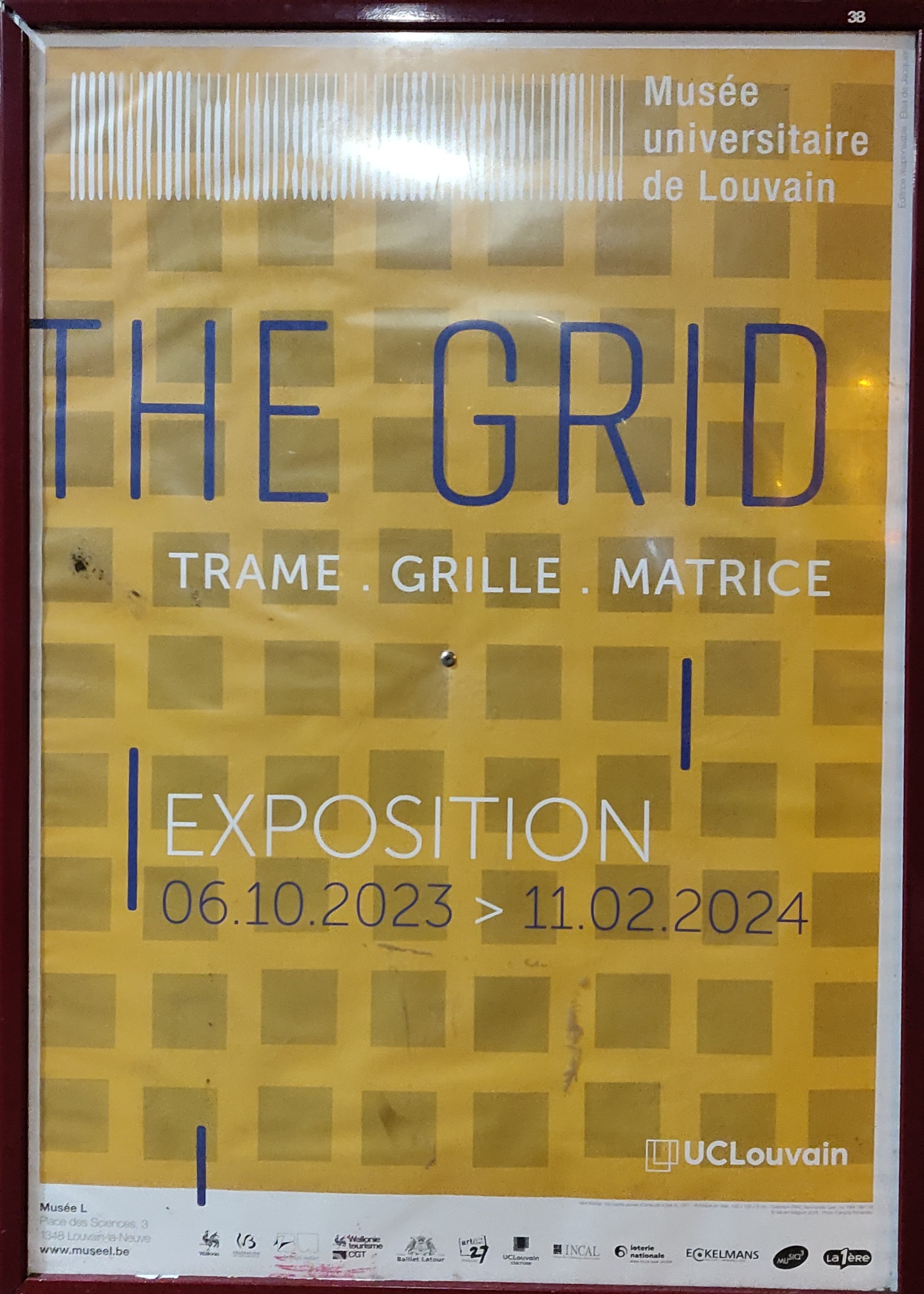
The Grid poster, in R

The MuseeL is the UCLouvain University museum in Louvain-la-Neuve. Highly recommended. It’s located to the lively place des sciences, in a nice brutalist style building, formerly the science university library. If you ever spend some time in Louvain-la-Neuve, do spare a couple of hours to visit it.

As an academic and an ‘amis du musée’, I can get in for free, and sometimes enjoy the quiet and rather unique atmosphere to get some work. The previous exhibition, named The Grid, was dedicated to the use of a grid in science. The poster and book of the exhibition, shown below, shows a grid, formed of smaller, slightly irregular squares. I thought this was a funny example to reproduce in R.

The first thing I need is the be able to draw squares. The plotSquare() function below plots on of width width at positions x and y.

plotSquare <- function(x, y, width) {
    x1 <- x - (width / 2)
    y1 <- y - (width / 2)
    x2 <- x1 + width
    y2 <- y1 + width
    rect(x1, y1, x2, y2)
}

Assuming I want an nsq by nsq grid of squares, below, I define that value to be 10, to draw a total of 100 squares.

## Number of squares
nsq <- 10

I also want some jitter, i.e. some random displacements from a perfect 10 by 10 alignment, set by the amount variables.

## amount of square jittering
amount <- 1.2

Finally, I need to define how much space is dedicated to the border between the squares.

## border ratio
ratio <- 0.2

Assuming that the grid will have a width and a height of 100 (arbitrary) unites, below I define the width sq_w of a square, considering the number of squares and the space that is dedicated to the border between squares. One I have the with of a square, I can compute the width border_w of the border between two squares.

sq_w <- (100 / nsq) * (1 - ratio)
border_w <- (100 - (nsq * sq_w)) / (nsq + 1)

I can now compute the x and y position of my squares. Given that my final grid is a square itself, these x and y positions apply to rows and columns of squares.

pos <- seq(border_w, 100 - border_w,
           length.out = nsq)

We can now produce the figure. I first define the margins of my plot with the par function: the margins have width 1 and outer margins 0. The plot() function doesn’t plot anything (`type = “n”), no axes, no frame, no labels. It however sets a grid itself, ranging from -2 to 100, to accommodate my squares and borders.

par(mar = rep(1, 4), oma = rep(0, 4))
plot(-2:(100 - border_w + 2), -2:(100 - border_w + 2),
     type = "n", xaxt = "n", yaxt = "n",
     xlab = "", ylab = "",
     frame.plot = FALSE)

The last step is to place the squares. The x and y positions are symmetrical, i.e defined by the pos variable above: the lines and columns are pos[1], pos[2], …, respectively, and the squares are added line by line, starting at line at pos[1]. A little amount of noise (defined by amount above) is added to the actual x and y position by the jitter() function.

for (y in pos) {
    pos_x <- jitter(rep(y, nsq), amount = amount)
    pos_y <- jitter(pos, amount = amount)
    plotSquare(pos_x, pos_y, sq_w)
}

The final output (with set.seed(123)), with the parameter above is show here.

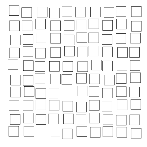
The full script is available here. The fun part is of course to play with the parameters, which is left as an exercise for the reader :-).