Chapter 11 Interactive visualisation

11.1 Interactivity graphs

This section is based on the on-line ggvis documentation

The goal of ggvis is to make it easy to build interactive graphics for exploratory data analysis. ggvis has a similar underlying theory to ggplot2 (the grammar of graphics), but it’s expressed a little differently, and adds new features to make your plots interactive. ggvis also incorporates shiny’s reactive programming model (see later) and dplyr’s grammar of data transformation.

library("ggvis")
sml <- sample(nrow(surveys_complete), 1e3)
surveys_sml <- surveys_complete[sml, ]

p <- ggvis(surveys_sml, x = ~weight, y = ~hindfoot_length)
p %>% layer_points()

surveys_sml %>%
    ggvis(x = ~weight, y = ~hindfoot_length,
          fill = ~species_id) %>%
    layer_points()

p %>% layer_points(fill = ~species_id)
p %>% layer_points(shape = ~species_id)

To set fixed plotting parameters, use :=.

p %>% layer_points(fill := "red", stroke := "black")
p %>% layer_points(size := 300, opacity := 0.4)
p %>% layer_points(shape := "cross")

11.1.1 Interactivity

p %>% layer_points(
          size := input_slider(10, 100),
          opacity := input_slider(0, 1))

p %>%
    layer_points() %>% 
    add_tooltip(function(df) df$weight)

• input_slider()
• input_checkbox()
• input_checkboxgroup()
• input_numeric()
• input_radiobuttons()
• input_select()
• input_text()

See the interactivity vignette for details.

11.1.2 Layers

Simple layers

• layer_points(), with properties x, y, shape, stroke, fill, strokeOpacity, fillOpacity, and opacity.
• layer_paths(), for paths and polygons (using the fill argument).
• layer_ribbons() for filled areas.
• layer_rects(), layer_text().

Compound layers, which which combine data transformations with one or more simple layers.

• layer_lines() which automatically orders by the x variable with arrange().
• layer_histograms() and layer_freqpolys(), which first bin the data with compute_bin().
• layer_smooths(), which fits and plots a smooth model to the data using compute_smooth().

See the layers vignette for details.

Like for ggplot2’s geoms, we can overly multiple layers:

p %>%
    layer_points() %>%
    layer_smooths(stroke := "red")

11.1.3 More components

• scales, to control the mapping between data and visual properties; see the properties and scales vignette.

• legends and axes to control the appearance of the guides produced by the scales. See the axes and legends vignette.

Challenge

Apply a PCA analysis on the iris data, and use ggvis to visualise that data along PC1 and PC2, controlling the point size using a slide bar.

11.2 Interactive apps

11.2.1 Introduction

This section is based on RStudio shiny tutorials.

From the shiny package website:

Shiny is an R package that makes it easy to build interactive web apps straight from R.

When using shiny, one tends to aim for more complete, long-lasting applications, rather then simply and transient visualisations.

A shiny application is composed of a ui (user interface) and a server that exchange information using a programming paradigm called reactive programming: changes performed by the user to the ui trigger a reaction by the server and the output is updated accordingly.

• In the ui: define the components of the user interface (such as page layout, page title, input options and outputs), i.e what the user will see and interact with.

• In the server: defines the computations in the R backend.

• The reactive programming is implemented through reactive functions, which are functions that are only called when their respective inputs are changed.

• An application is run with the shiny::runApp() function, which takes the directory containing the two files as input.

Before looking at the details of such an architecture, let’s build a simple example from scratch, step by step. This app, shown below, uses the faithful data, describing the wainting time between eruptions and the duration of the reuption for the Old Faithful geyser in Yellowstone National Park, Wyoming, USA.

head(faithful)

##   eruptions waiting
## 1     3.600      79
## 2     1.800      54
## 3     3.333      74
## 4     2.283      62
## 5     4.533      85
## 6     2.883      55

It shows the distribution of waiting times along a histogram (produced by the hist function) and provides a slider to adjust the number of bins (the breaks argument to hist).

The app can also be opened at https://lgatto.shinyapps.io/shiny-app1/

11.2.2 Creation of our fist shiny app

1. Create a directory that will contain the app, such as for example "shinyapp".
2. In this directory, create the ui and server files, named ui.R and server.R.
3. In the ui.R file, let’s defines a (fluid) page containing

• a title panel with a page title;
• a layout containing a sidebar and a main panel

library(shiny)

shinyUI(fluidPage(
    titlePanel("My Shiny App"),
    sidebarLayout(
        sidebarPanel(
        ),
        mainPanel(
        )
    )
))

4. In the server.R file, we define the shinyServer function that handles input and ouputs (none at this stage) and the R logic.

library(shiny)

shinyServer(function(input, output) {
})

5. Let’s now add some items to the ui: a text input widget in the sidebar and a field to hold the text ouput.

library(shiny)

shinyUI(fluidPage(
    titlePanel("My Shiny App"),
    sidebarLayout(
        sidebarPanel(
            textInput("textInput", "Enter text here:")
        ),
        mainPanel(
            textOutput("textOutput")
        )
    )
))

6. In the server.R file, we add in the shinyServer function some R code defining how to manipulate the user-provided text and render it using a shiny textOuput.

library(shiny)

shinyServer(function(input, output) {
    output$textOutput <- renderText(paste("User-entered text: ",
                                          input$textInput))
})

7. Let’s now add a plot in the main panel in ui.R and some code to draw a histogram in server.R:

library(shiny)

shinyUI(fluidPage(
    titlePanel("My Shiny App"),
    sidebarLayout(
        sidebarPanel(
            textInput("textInput", "Enter text here:")
        ),
        mainPanel(
            textOutput("textOutput"),
            plotOutput("distPlot")            
        )
    )
))

library(shiny)

shinyServer(function(input, output) {
    output$textOutput <- renderText(paste("User-entered text: ",
                                          input$textInput))
    output$distPlot <- renderPlot({
        x    <- faithful[, 2]
        hist(x)
    })
    
})

8. We want to be able to control the number of breaks used to plot the histograms. We first add a sliderInput to the ui for the user to specify the number of bins, and then make use of that new input to parametrise the histogram.

library(shiny)

shinyUI(fluidPage(
    titlePanel("My Shiny App"),
    sidebarLayout(
        sidebarPanel(
            textInput("textInput", "Enter text here:"),
            sliderInput("bins",
                        "Number of bins:",
                        min = 1,
                        max = 50,
                        value = 30)            
        ),
        mainPanel(
            textOutput("textOutput"),
            plotOutput("distPlot")            
        )
    )
))

library(shiny)

shinyServer(function(input, output) {
    output$textOutput <- renderText(paste("User-entered text: ",
                                          input$textInput))
    output$distPlot <- renderPlot({
        x    <- faithful[, 2]
        bins <- seq(min(x), max(x), length.out = input$bins + 1)    
        hist(x, breaks = bins)
    })
    
})

9. The next addition is to add a menu for the user to choose a set of predefined colours (that would be a selectInput) in the ui.R file and use that new input to parametrise the colour of the histogramme in the server.R file.

library(shiny)

shinyUI(fluidPage(
    titlePanel("My Shiny App"),
    sidebarLayout(
        sidebarPanel(
            textInput("textInput", "Enter text here:"),
            sliderInput("bins",
                        "Number of bins:",
                        min = 1,
                        max = 50,
                        value = 30),
            selectInput("col", "Select a colour:",
                        choices = c("steelblue", "darkgray", "orange"))            
        ),
        mainPanel(
            textOutput("textOutput"),
            plotOutput("distPlot")
        )
    )
))

library(shiny)

shinyServer(function(input, output) {
    output$textOutput <- renderText(paste("User-entered text: ",
                                          input$textInput))
    output$distPlot <- renderPlot({
        x    <- faithful[, 2]
        bins <- seq(min(x), max(x), length.out = input$bins + 1)
        hist(x, breaks = bins, col = input$col)
    })
    
})

10. The last addition that we want is to visualise the actual data in the main panel. We add a dataTableOutput in ui.R and generate that table in server.R using a renderDataTable rendering function.

library(shiny)
## Define UI for application that draws a histogram
shinyUI(fluidPage(
    ## Application title
    titlePanel("My Shiny App"),
    ## Sidebar with text, slide bar and menu selection inputs
    sidebarLayout(
        sidebarPanel(
            textInput("textInput", "Enter text here:"),
            sliderInput("bins",
                        "Number of bins:",
                        min = 1,
                        max = 50,
                        value = 30),
            selectInput("col", "Select a colour:",
                        choices = c("steelblue", "darkgray", "orange"))
        ),
        ## Main panel showing user-entered text, a reactive plot and a
        ## dynamic table
        mainPanel(
            textOutput("textOutput"),
            plotOutput("distPlot"),
            dataTableOutput("dataTable")
        )
    )
))

library(shiny)
## Define server logic 
shinyServer(function(input, output) {
    output$textOutput <- renderText(paste("User-entered text: ",
                                          input$textInput))
    ## Expression that generates a histogram. The expression is
    ## wrapped in a call to renderPlot to indicate that:
    ##
    ##  1) It is "reactive" and therefore should be automatically
    ##     re-executed when inputs change
    ##  2) Its output type is a plot
    output$distPlot <- renderPlot({
        x    <- faithful[, 2]  ## Old Faithful Geyser data
        bins <- seq(min(x), max(x), length.out = input$bins + 1)
        ## draw the histogram with the specified number of bins
        hist(x, breaks = bins, col = input$col, border = 'white')
    })
    output$dataTable <- renderDataTable(faithful)
})

Challenge

Write and your shinyapp applications, as described above.

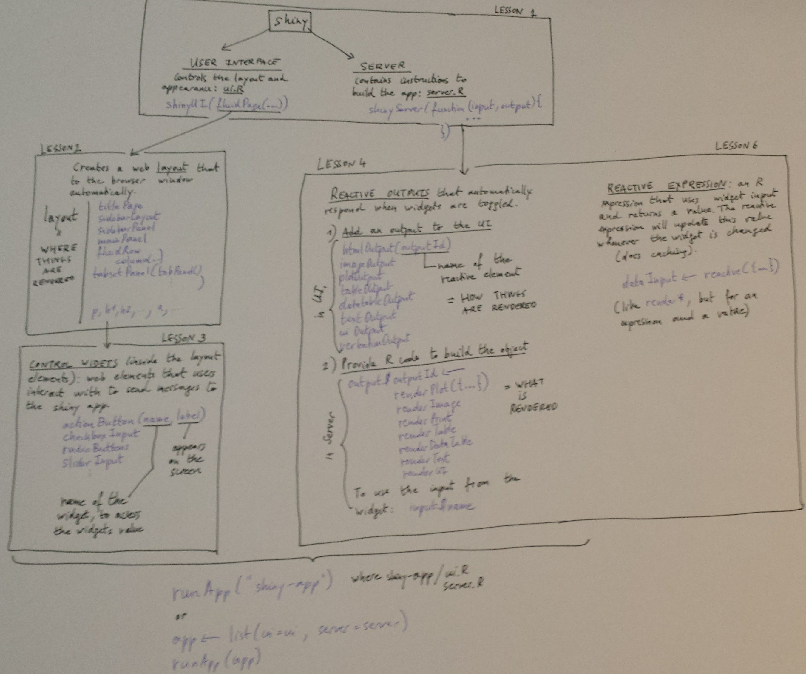
11.2.3 The shiny infrastructure

The overview figure below is based and makes reference to lessons of the written tutorial.

11.2.4 Another shiny app

The ui uses the fluidPage UI and a sidebar layout. The sidebar panel contains a textInput with a caption, a selectInput to choose from the three possible datasets rock, pressure or cars, and a numericInput to define how many observations to show.

The main panel use a textOutput to display the caption, a verbatimOutput to show the output of the summary function on the data chosen in the selectInput above, and a tableOutput to show the head of that same data.

library("shiny")
# Define UI for dataset viewer application
shinyUI(fluidPage(
  # Application title
  titlePanel("Reactivity"),
  # Sidebar with controls to provide a caption, select a dataset,
  # and specify the number of observations to view. Note that
  # changes made to the caption in the textInput control are
  # updated in the output area immediately as you type
  sidebarLayout(
    sidebarPanel(
      textInput("caption", "Caption:", "Data Summary"),
      selectInput("dataset", "Choose a dataset:", 
                  choices = c("rock", "pressure", "cars")),
      numericInput("obs", "Number of observations to view:", 10)
    ),
    # Show the caption, a summary of the dataset and an HTML 
   # table with the requested number of observations
    mainPanel(
      h3(textOutput("caption", container = span)),
      verbatimTextOutput("summary"), 
      tableOutput("view")
    )
  )
))

The server defines a reactive expression that sets the appropriate data based on the selectInput above. It produces three outputs:

1. the caption using renderText and the caption defined above;
2. the appropriate summary using renderPrint and the reactive data;
3. the table using renderTable to produce the head with the reactive data and number of observations defined by the numbericInput above.

library(shiny)
library(datasets)
# Define server logic required to summarize and view the selected
# dataset
shinyServer(function(input, output) {
  # By declaring datasetInput as a reactive expression we ensure 
  # that:
  #
  #  1) It is only called when the inputs it depends on changes
  #  2) The computation and result are shared by all the callers 
  #   (it only executes a single time)
  #
  datasetInput <- reactive({
    switch(input$dataset,
           "rock" = rock,
           "pressure" = pressure,
           "cars" = cars)
  })
  # The output$caption is computed based on a reactive expression
  # that returns input$caption. When the user changes the
  # "caption" field:
  #
  #  1) This function is automatically called to recompute the 
  #     output 
  #  2) The new caption is pushed back to the browser for 
  #     re-display
  # 
  # Note that because the data-oriented reactive expressions
  # below don't depend on input$caption, those expressions are
  # NOT called when input$caption changes.
  output$caption <- renderText({
    input$caption
  })
  # The output$summary depends on the datasetInput reactive
  # expression, so will be re-executed whenever datasetInput is
  # invalidated
  # (i.e. whenever the input$dataset changes)
  output$summary <- renderPrint({
    dataset <- datasetInput()
    summary(dataset)
  })
  # The output$view depends on both the databaseInput reactive
  # expression and input$obs, so will be re-executed whenever
  # input$dataset or input$obs is changed. 
  output$view <- renderTable({
    head(datasetInput(), n = input$obs)
  })
})

Challenge

Using the code above, implement and run the app.

11.2.5 Single-file app

Instead of defining the ui and server in their respective files, they can be combined into list to be passed directly to runApp:

ui <- fluidPage(...)
server <- function(input, output) { ... }

app <- list(ui = ui, server = server)
runApp(app)

Challenges

1. Create an app to visualise the iris data where the user can select along which features to view the data.

2. As above, where the visualisation is a PCA plot and the user chooses the PCs.

11.2.6 There’s more to shiny

11.2.6.1 Sharing shiny apps

• Share the code file(s) and runApp
• runUrl
• runGitHub
• runGist
• shinyapps
• Shiny server (in-house)

11.2.6.2 More interactivity

 plotOutput("pca",
            hover = "hover",
            click = "click",
            dblclick = "dblClick",
            brush = brushOpts(
                id = "brush",
                resetOnNew = TRUE))

Example here.

11.2.6.3 References

• shiny page
• shiny cheat sheet