Chapter 10 Visualisation of high-dimensional data in R
This section is based composed of the Visualisation of high-dimensional data presentation, and parts of the Introduction to Machine Learning with R course (unsupervised learning chapter).
10.1 Introduction
10.2 Data
To illustrate some visualisation techniques, we are going to make use of Edgar Anderson’s Iris Data, available in R with
data(iris)From the iris manual page:
This famous (Fisher’s or Anderson’s) iris data set gives the measurements in centimeters of the variables sepal length and width and petal length and width, respectively, for 50 flowers from each of 3 species of iris. The species are Iris setosa, versicolor, and virginica.


For more details, see ?iris.
10.3 K-means clustering
The k-means clustering algorithms aims at partitioning n observations into a fixed number of k clusters. The algorithm will find homogeneous clusters.
In R, we use
stats::kmeans(x, centers = 3, nstart = 10)where
xis a numeric data matrixcentersis the pre-defined number of clusters- the k-means algorithm has a random component and can be repeated
nstarttimes to improve the returned model
Challenge:
- To learn about k-means, let’s use the
iriswith the sepal and petal length variables only (to facilitate visualisation). Create such a data matrix and name itx
- Run the k-means algorithm on the newly generated data
x, save the results in a new variablecl, and explore its output when printed.
- The actual results of the algorithms, i.e. the cluster membership can be accessed in the
clusterselement of the clustering result output. Use it to colour the inferred clusters to generate a figure like shown below.
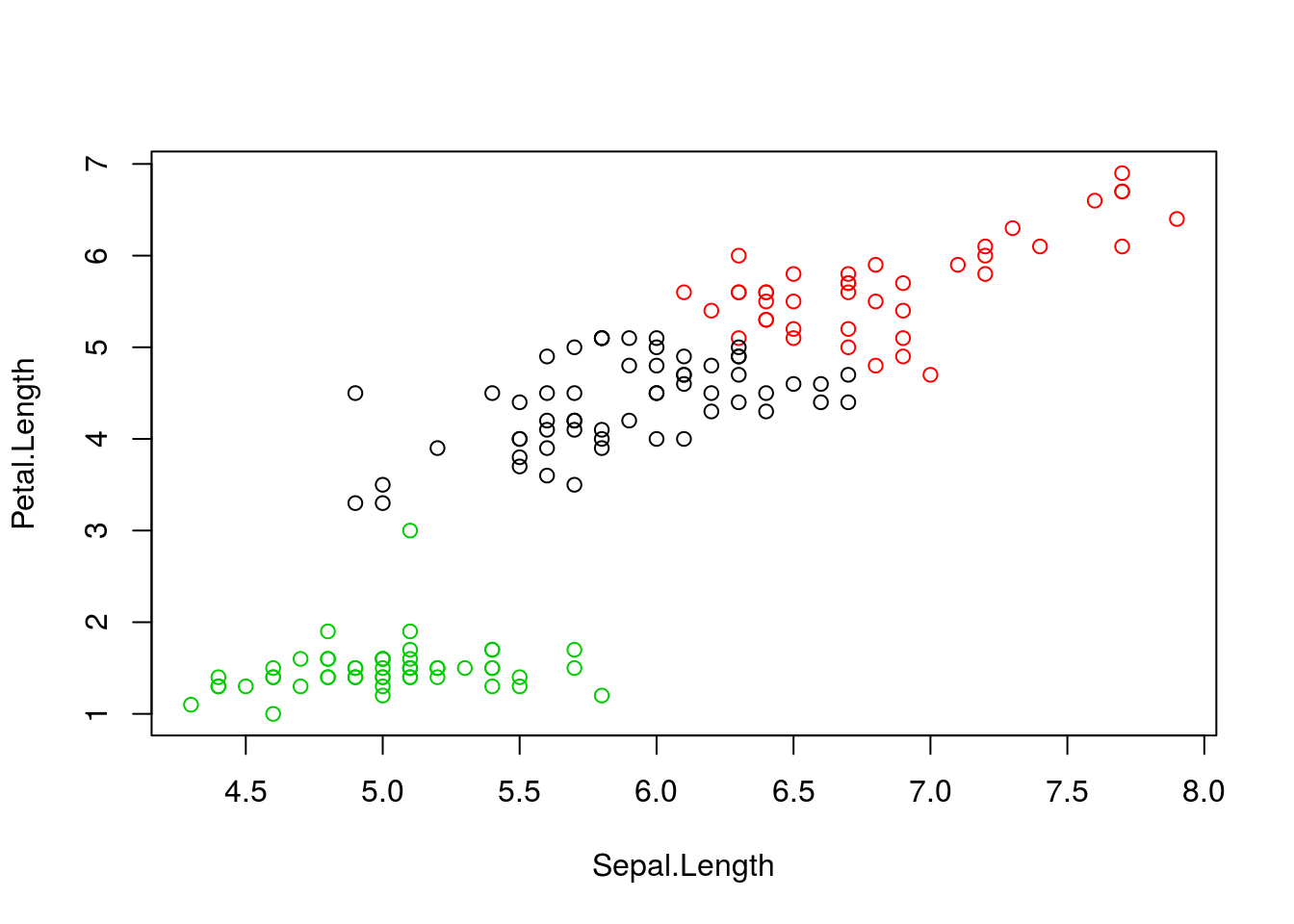
Figure 10.1: k-means algorithm on sepal and petal lengths
i <- grep("Length", names(iris))
x <- iris[, i]
cl <- kmeans(x, 3, nstart = 10)
plot(x, col = cl$cluster)
10.3.1 How does k-means work
Initialisation: randomly assign class membership
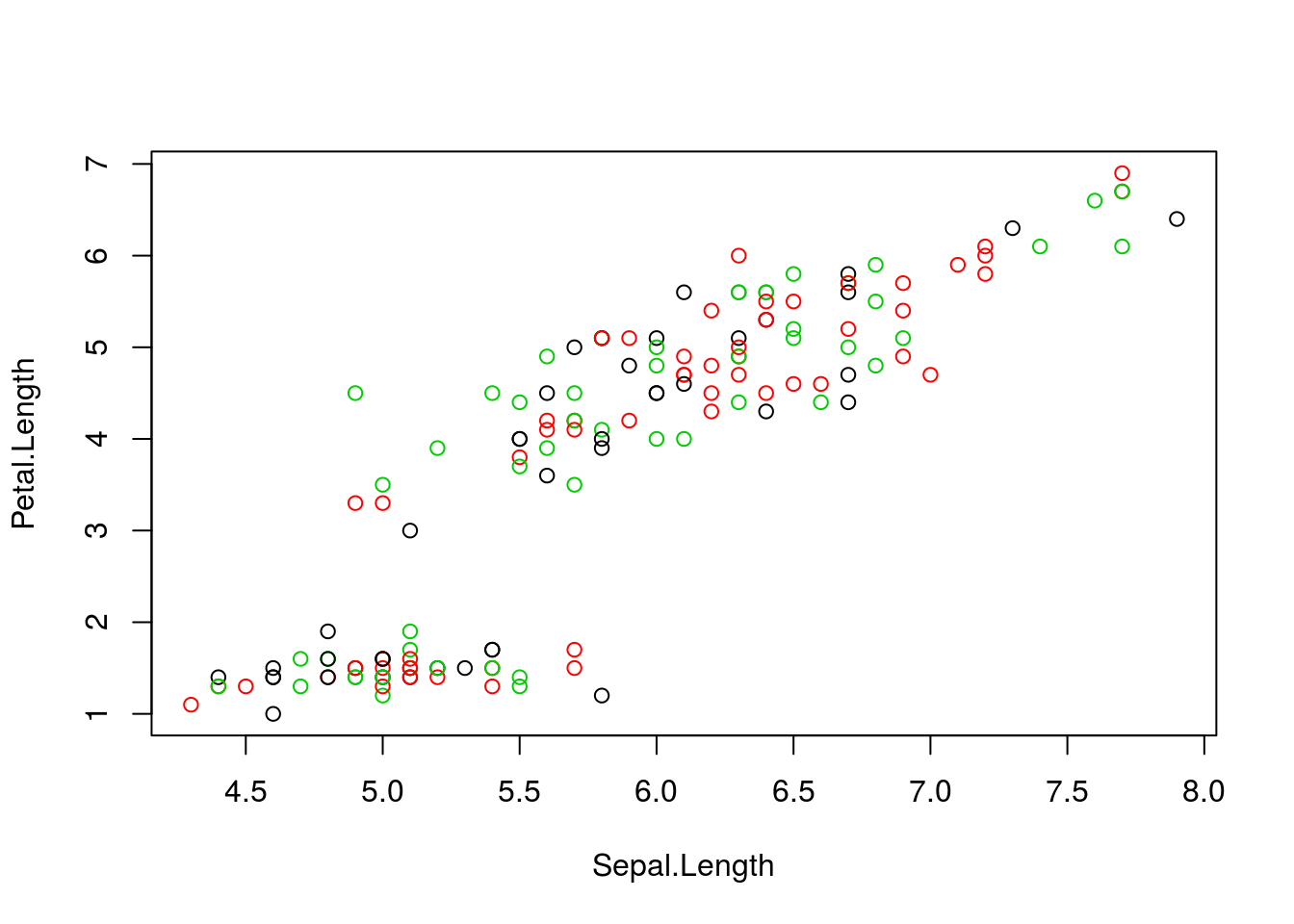
Figure 10.2: k-means random intialisation
Iteration:
- Calculate the centre of each subgroup as the average position of all observations is that subgroup.
- Each observation is then assigned to the group of its nearest centre.
It’s also possible to stop the algorithm after a certain number of iterations, or once the centres move less than a certain distance.
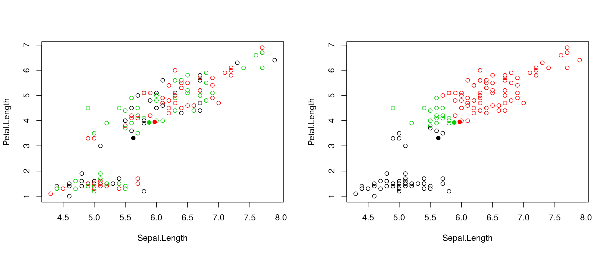
Figure 10.3: k-means iteration: calculate centers (left) and assign new cluster membership (right)
Termination: Repeat iteration until no point changes its cluster membership.

k-means convergence (credit Wikipedia)
10.3.2 Model selection
Due to the random initialisation, one can obtain different clustering results. When k-means is run multiple times, the best outcome, i.e. the one that generates the smallest total within cluster sum of squares (SS), is selected. The total within SS is calculated as:
For each cluster results:
- for each observation, determine the squared euclidean distance from observation to centre of cluster
- sum all distances
Note that this is a local minimum; there is no guarantee to obtain a global minimum.
Challenge:
Repeat kmeans on our
xdata multiple times, setting the number of iterations to 1 or greater and check whether you repeatedly obtain the same results. Try the same with random data of identical dimensions.
cl1 <- kmeans(x, centers = 3, nstart = 10)
cl2 <- kmeans(x, centers = 3, nstart = 10)
table(cl1$cluster, cl2$cluster)
##
## 1 2 3
## 1 58 0 0
## 2 0 41 0
## 3 0 0 51cl1 <- kmeans(x, centers = 3, nstart = 1)
cl2 <- kmeans(x, centers = 3, nstart = 1)
table(cl1$cluster, cl2$cluster)##
## 1 2 3
## 1 0 0 41
## 2 0 51 0
## 3 58 0 0set.seed(42)
xr <- matrix(rnorm(prod(dim(x))), ncol = ncol(x))
cl1 <- kmeans(xr, centers = 3, nstart = 1)
cl2 <- kmeans(xr, centers = 3, nstart = 1)
table(cl1$cluster, cl2$cluster)##
## 1 2 3
## 1 46 0 6
## 2 1 51 0
## 3 0 1 45diffres <- cl1$cluster != cl2$cluster
par(mfrow = c(1, 2))
plot(xr, col = cl1$cluster, pch = ifelse(diffres, 19, 1))
plot(xr, col = cl2$cluster, pch = ifelse(diffres, 19, 1))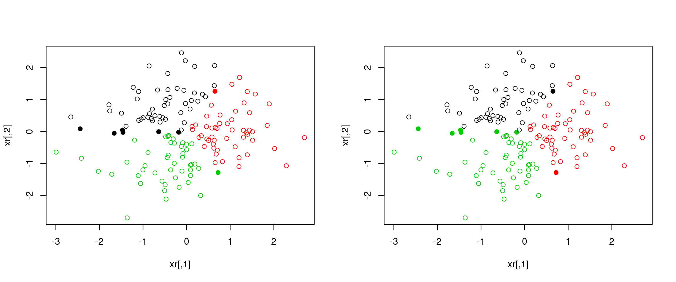
Figure 10.4: Different k-means results on the same (random) data
10.3.3 How to determine the number of clusters
- Run k-means with
k=1,k=2, …,k=n - Record total within SS for each value of k.
- Choose k at the elbow position, as illustrated below.
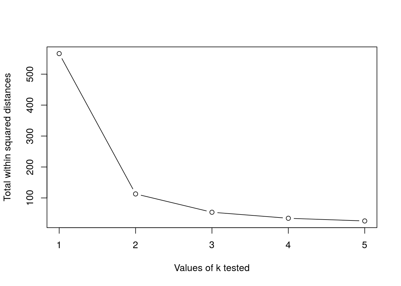
Challenge
Calculate the total within sum of squares for k from 1 to 5 for our
xtest data, and reproduce the figure above.
ks <- 1:5
tot_within_ss <- sapply(ks, function(k) {
    cl <- kmeans(x, k, nstart = 10)
    cl$tot.withinss
})
plot(ks, tot_within_ss, type = "b")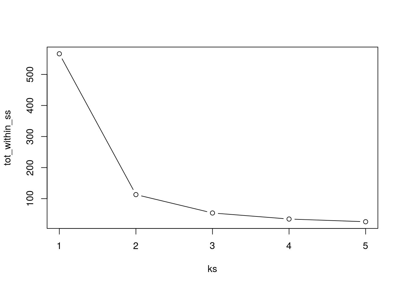
10.4 Hierarchical clustering
10.4.1 How does hierarchical clustering work
Initialisation: Starts by assigning each of the n point its own cluster
Iteration
- Find the two nearest clusters, and join them together, leading to n-1 clusters
- Continue merging cluster process until all are grouped into a single cluster
Termination: All observations are grouped within a single cluster.
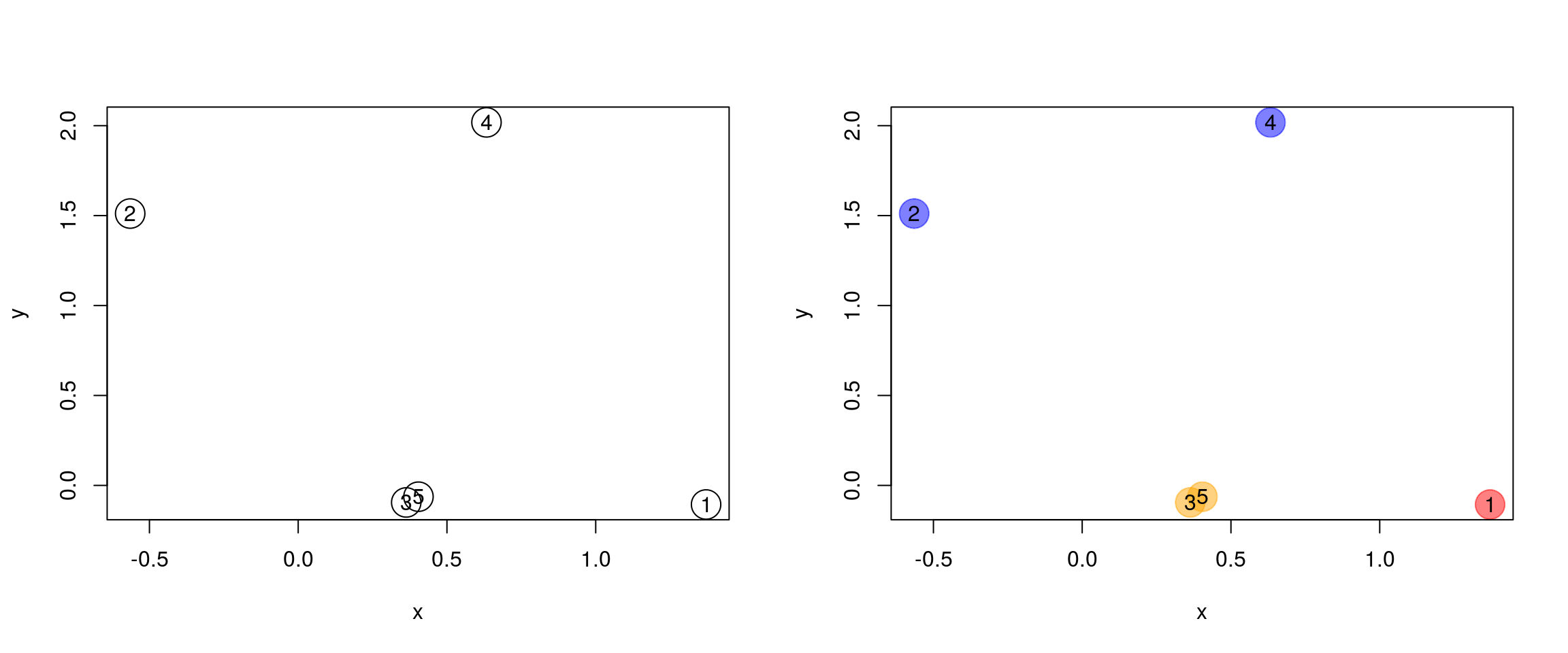
Figure 10.5: Hierarchical clustering: initialisation (left) and colour-coded results after iteration (right).
The results of hierarchical clustering are typically visualised along a dendrogram, where the distance between the clusters is proportional to the branch lengths.
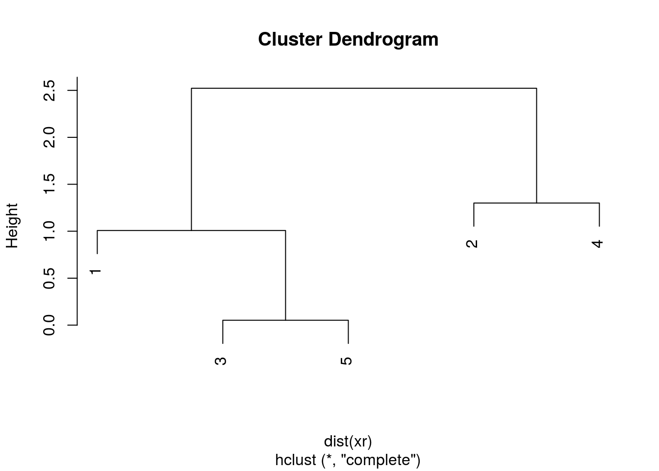
Figure 10.6: Visualisation of the hierarchical clustering results on a dendrogram
In R:
- Calculate the distance using
dist, typically the Euclidean distance. - Hierarchical clustering on this distance matrix using
hclust
Challenge
Apply hierarchical clustering on the
irisdata and generate a dendrogram using the dedicatedplotmethod.
d <- dist(iris[, 1:4])
hcl <- hclust(d)
hcl
##
## Call:
## hclust(d = d)
##
## Cluster method : complete
## Distance : euclidean
## Number of objects: 150plot(hcl)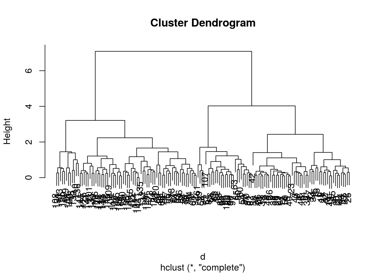
10.4.2 Defining clusters
After producing the hierarchical clustering result, we need to cut the tree (dendrogram) at a specific height to defined the clusters. For example, on our test dataset above, we could decide to cut it at a distance around 1.5, with would produce 2 clusters.
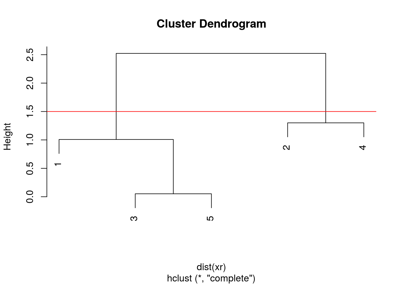
Figure 10.7: Cutting the dendrogram at height 1.5.
In R we can us the cutree function to
- cut the tree at a specific height:
cutree(hcl, h = 1.5) - cut the tree to get a certain number of clusters:
cutree(hcl, k = 2)
Challenge
- Cut the iris hierarchical clustering result at a height to obtain 3 clusters by setting
h.- Cut the iris hierarchical clustering result at a height to obtain 3 clusters by setting directly
k, and verify that both provide the same results.
plot(hcl)
abline(h = 3.9, col = "red")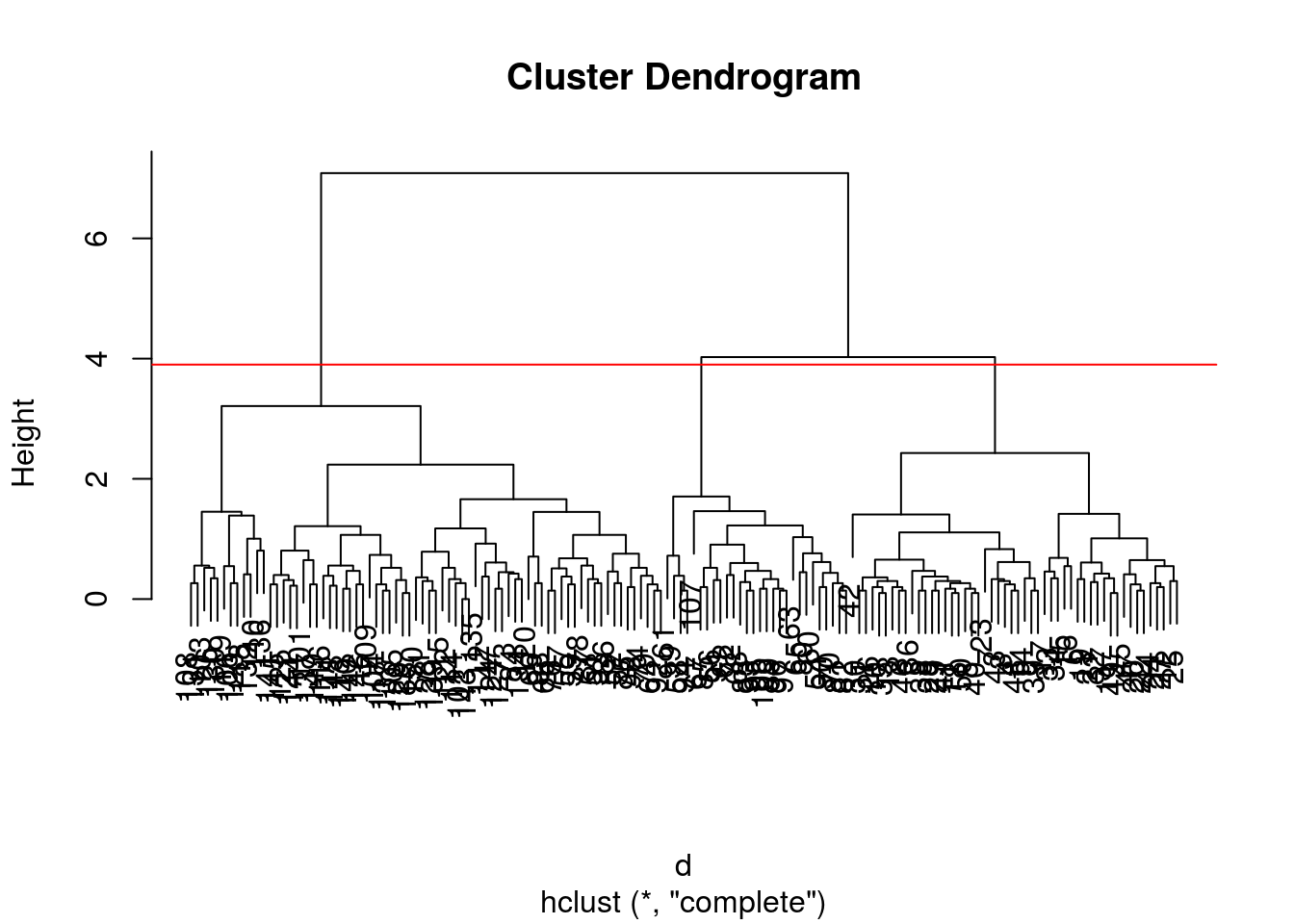
cutree(hcl, k = 3)## [1] 1 1 1 1 1 1 1 1 1 1 1 1 1 1 1 1 1 1 1 1 1 1 1 1 1 1 1 1 1 1 1 1 1 1 1
## [36] 1 1 1 1 1 1 1 1 1 1 1 1 1 1 1 2 2 2 3 2 3 2 3 2 3 3 3 3 2 3 2 3 3 2 3
## [71] 2 3 2 2 2 2 2 2 2 3 3 3 3 2 3 2 2 2 3 3 3 2 3 3 3 3 3 2 3 3
## [ reached getOption("max.print") -- omitted 50 entries ]cutree(hcl, h = 3.9)## [1] 1 1 1 1 1 1 1 1 1 1 1 1 1 1 1 1 1 1 1 1 1 1 1 1 1 1 1 1 1 1 1 1 1 1 1
## [36] 1 1 1 1 1 1 1 1 1 1 1 1 1 1 1 2 2 2 3 2 3 2 3 2 3 3 3 3 2 3 2 3 3 2 3
## [71] 2 3 2 2 2 2 2 2 2 3 3 3 3 2 3 2 2 2 3 3 3 2 3 3 3 3 3 2 3 3
## [ reached getOption("max.print") -- omitted 50 entries ]identical(cutree(hcl, k = 3), cutree(hcl, h = 3.9))## [1] TRUEChallenge
Using the same value
k = 3, verify if k-means and hierarchical clustering produce the same results on theirisdata.Which one, if any, is correct?
km <- kmeans(iris[, 1:4], centers = 3, nstart = 10)
hcl <- hclust(dist(iris[, 1:4]))
table(km$cluster, cutree(hcl, k = 3))
##
## 1 2 3
## 1 0 38 0
## 2 50 0 0
## 3 0 34 28par(mfrow = c(1, 2))
plot(iris$Petal.Length, iris$Sepal.Length, col = km$cluster, main = "k-means")
plot(iris$Petal.Length, iris$Sepal.Length, col = cutree(hcl, k = 3), main = "Hierarchical clustering")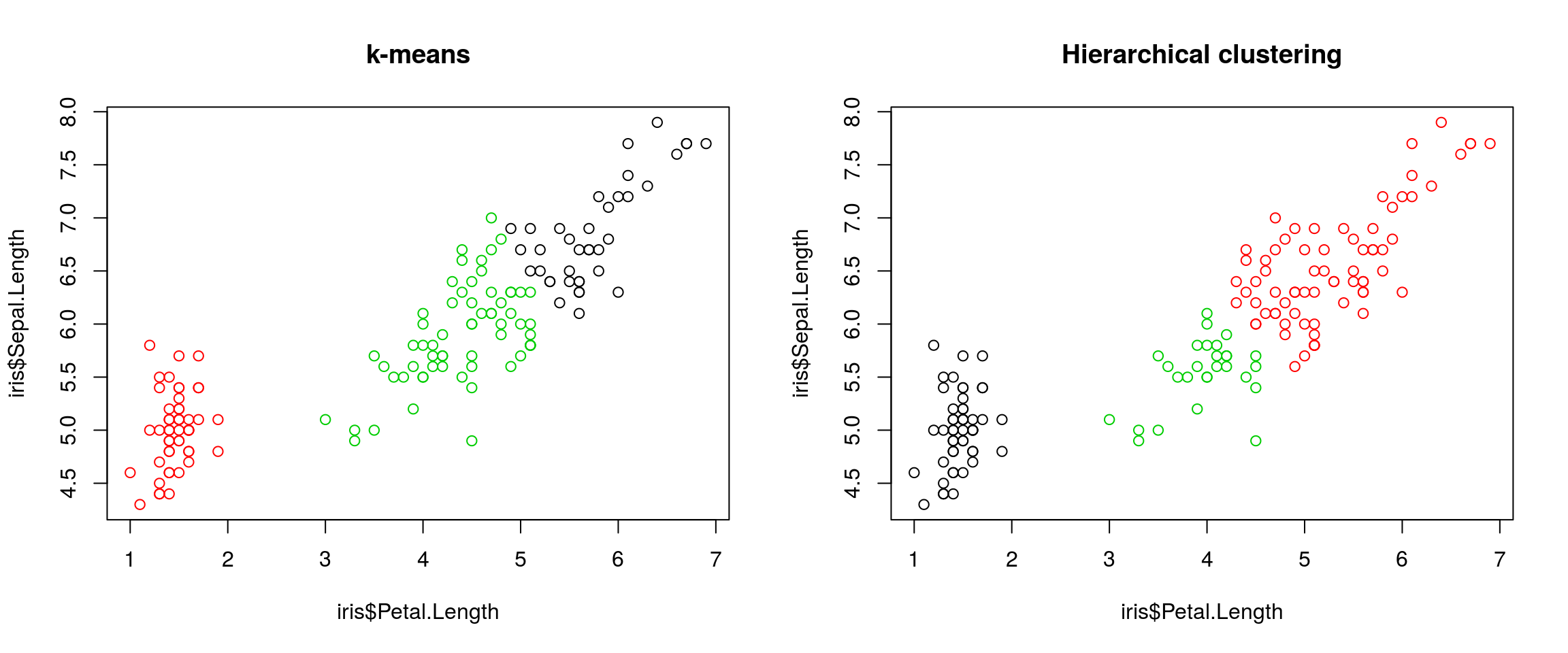
## Checking with the labels provided with the iris data
table(iris$Species, km$cluster)
##
## 1 2 3
## setosa 0 50 0
## versicolor 2 0 48
## virginica 36 0 14table(iris$Species, cutree(hcl, k = 3))##
## 1 2 3
## setosa 50 0 0
## versicolor 0 23 27
## virginica 0 49 110.5 Principal component analysis (PCA)
In R, we can use the prcomp function.
Let’s explore PCA on the iris data. While it contains only 4 variables, is already becomes difficult to visualise the 3 groups along all these dimensions.
pairs(iris[, -5], col = iris[, 5], pch = 19)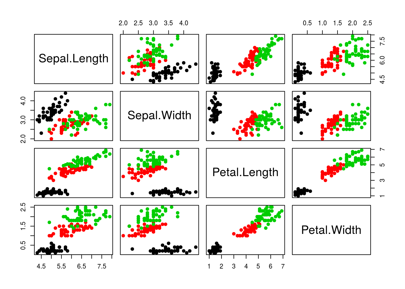
Let’s use PCA to reduce the dimension.
irispca <- prcomp(iris[, -5])
summary(irispca)
## Importance of components:
## PC1 PC2 PC3 PC4
## Standard deviation 2.0563 0.49262 0.2797 0.15439
## Proportion of Variance 0.9246 0.05307 0.0171 0.00521
## Cumulative Proportion 0.9246 0.97769 0.9948 1.00000A summary of the prcomp output shows that along PC1 along, we are able to retain over 92% of the total variability in the data.
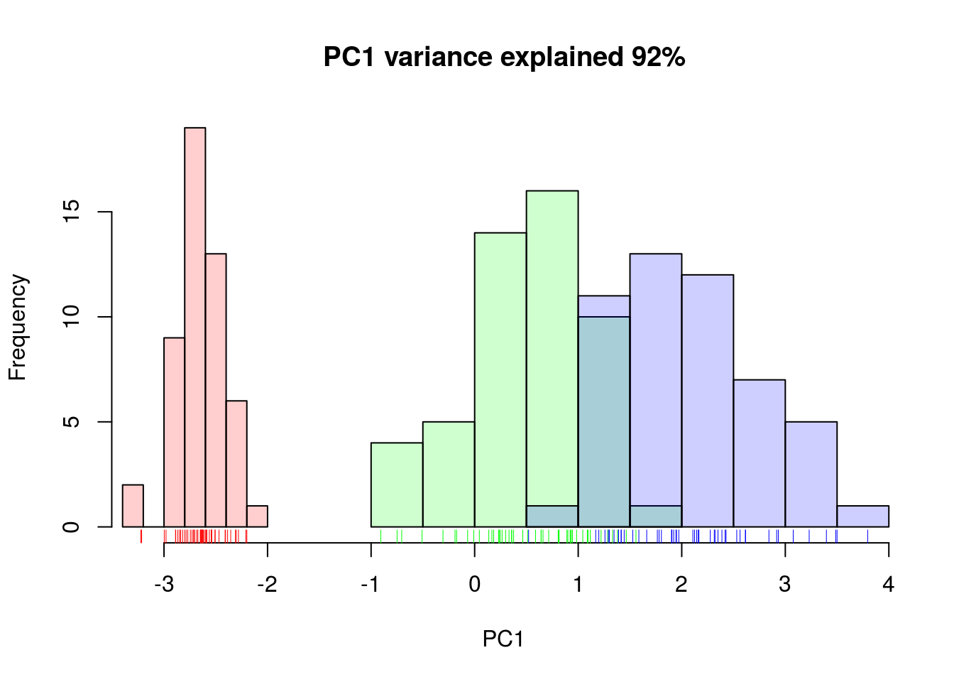
Figure 10.8: Iris data along PC1.
10.5.1 Visualisation
A biplot features all original points re-mapped (rotated) along the first two PCs as well as the original features as vectors along the same PCs. Feature vectors that are in the same direction in PC space are also correlated in the original data space.
biplot(irispca)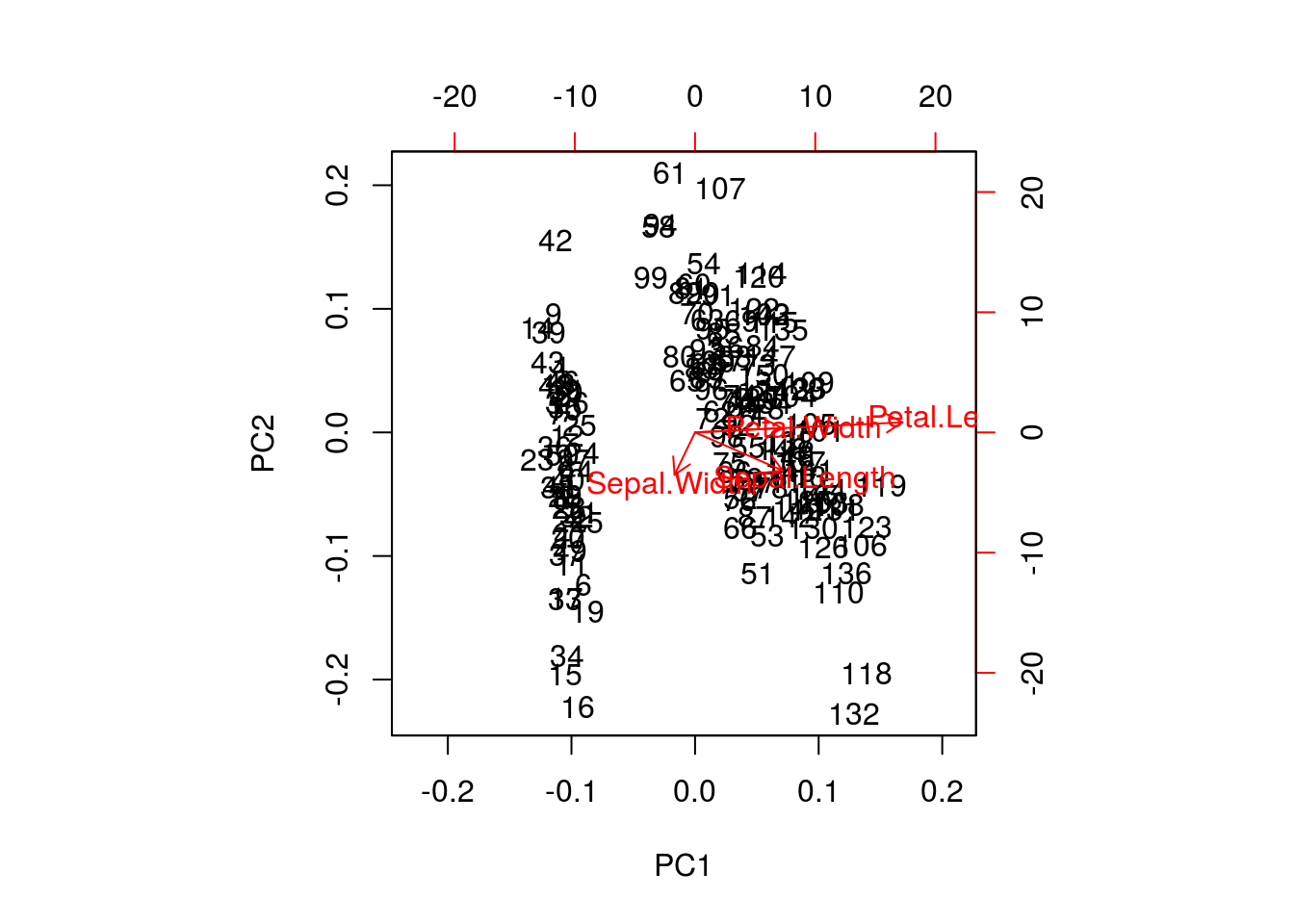
One important piece of information when using PCA is the proportion of variance explained along the PCs, in particular when dealing with high dimensional data, as PC1 and PC2 (that are generally used for visualisation), might only account for an insufficient proportion of variance to be relevant on their own.
In the code chunk below, I extract the standard deviations from the PCA result to calculate the variances, then obtain the percentage of and cumulative variance along the PCs.
var <- irispca$sdev^2
(pve <- var/sum(var))
## [1] 0.924618723 0.053066483 0.017102610 0.005212184cumsum(pve)## [1] 0.9246187 0.9776852 0.9947878 1.0000000Challenge
- Repeat the PCA analysis on the iris dataset above, reproducing the biplot and preparing a barplot of the percentage of variance explained by each PC.
- It is often useful to produce custom figures using the data coordinates in PCA space, which can be accessed as
xin theprcompobject. Reproduce the PCA plots below, along PC1 and PC2 and PC3 and PC4 respectively.
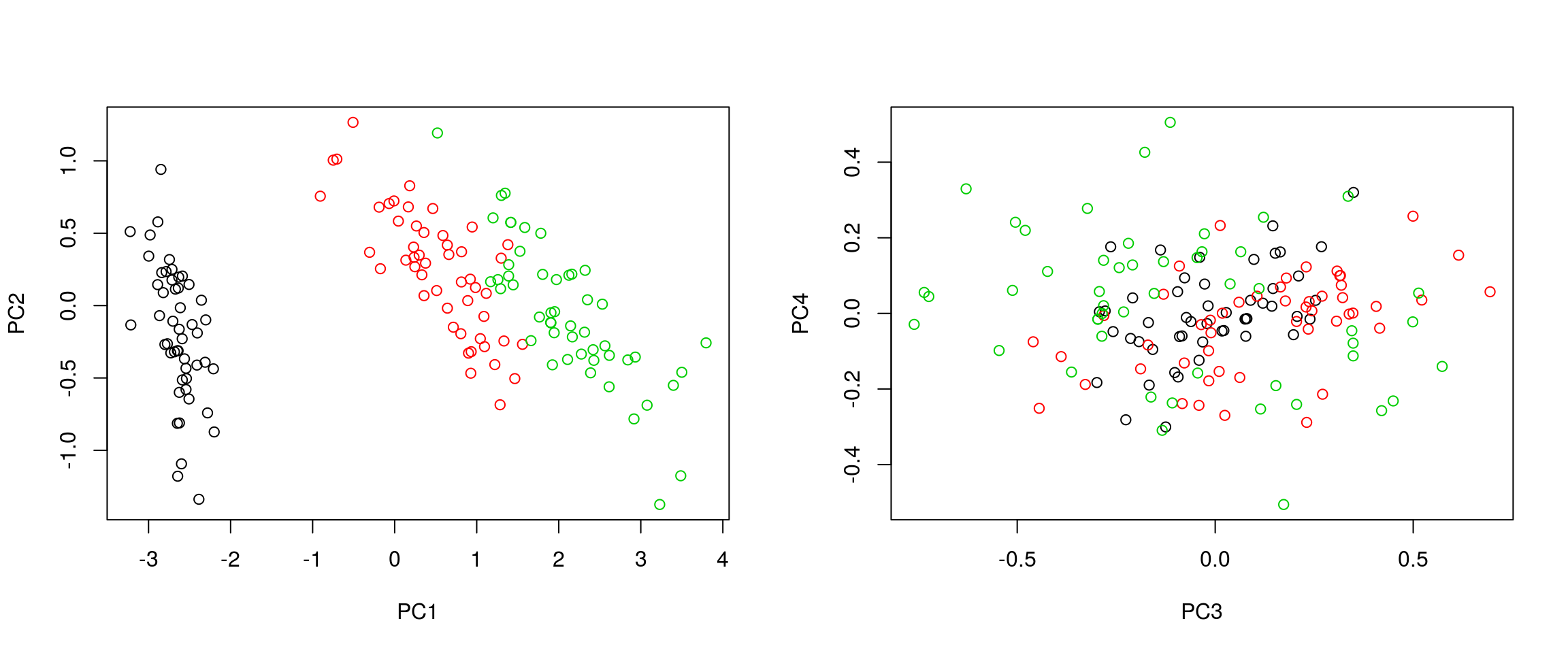
par(mfrow = c(1, 2))
plot(irispca$x[, 1:2], col = iris$Species)
plot(irispca$x[, 3:4], col = iris$Species)