Chapter 12 Navigating the Bioconductor project
12.1 biocViews
Bioconductor has become a large project proposing many packages (1473 software packages at the time of writing) across many domains of high throughput biology. It continues to grow, at an increasing rate, and it can be difficult to get started.
One way to find packages of interest is to navigate the biocViews hierarchy. Every package is tagged with a set of biocViews labels. The highest level defines 3 types of packages:
- Software: packages providing a specific functionality.
- AnnotationData: packages providing annotations, such as various ontologies, species annotations, microarray annotations, …
- ExperimentData: packages distributing experiments.
The biocViews page is available here
It is most easily accessed by clicking on the software packages link on the homepage, under About Bioconductor.
See also this page for additional information.
12.2 Workflows
On the other hand, people generally don’t approach the Bioconductor project to learn the whole project, but are interested by a specific analysis from a Bioconductor package, that they have read in a paper of interest. In my opinion, it is more effective to restrict ones attention to a problem or analysis of interest to first immerse oneself into Bioconductor, then broaden up ones experience to other topics and packages.
To to that, the project offers workflows that provide a general introduction to topics such as sequence analysis, annotation resources, RNA-Seq data analyis, Mass spectrometry and proteomics, CyTOF analysis, ….
A similar set of resources are published in F1000Research under the Bioconductor gateway
These peer-reviewed papers describe more complete pipelines involving one or several packages.
12.3 Learning about specific packages
Each Bioconductor package has it’s own landing pages that provides all necessary information about a package, including a short summary, its current version, the authors, how the cite the package, installation instructions, and links to all package vignettes.
Any Bioconductor package page can be contructed by appending the package’s name to https://bioconductor.org/packages/ to produce an URL like
This works for any type of package (software, annotation or data). For example, the pages for packages DESeq2 or MSnbase would be
and
These short URLs are then resolved to their longer form to redirect to the longer package URL leading the user to the current release version of the packge.
12.3.1 Package vignettes
An important quality of every Bioconductor package is the availability of a dedicated vignette. Vignettes are documentations (generally provided as pdf or html files) that provide a generic overview of the package, without necessarily going in detail for every function of the package.
Vignettes are special in that respect as they are produced as part of the package building process. The code in a vignette is executed and its output, whether in the form of simple text, tables and figures, are inserted in the vignette before the final file (in pdf or html) is produced. Hence, all the code and outputs are guaranteed to be correct and reproduced.
Given a vignette, it is this possible to re-generate all the results. To make reproducing a long vignette as easy as possible without copy and pasting all code chunks one by one, it is possible to extract the code into an R script runnung the Stangle (from the utils package - see here for details) or knitr::purl functions on the vignette source document.
12.3.2 Installation
The installation of a Bioconductor package is done using the biocLite function from the BiocInstaller package. The first time, when the package isn’t available yet, you need to run
## try http:// if https:// URLs are not supported
source("https://bioconductor.org/biocLite.R")
The above command will install and load BiocInstaller. If it isn’t loaded yet, first load it with library, then install your package(s) of interest with biocLite:
library("BiocInstaller")
biocLite("Biobase")
This page provides more details on package installation and update.
12.4 Versions
It is also useful to know that at any given time, there are two Bioconductor versions - there is always a release (stable) and a development (devel) versions. For example, in October 2017, the release version is 3.6 and the development is 3.7.
The individual packages have a similar scheme. Every package is available for the release and the development versions of Bioconductor. These two versions of the package have also different version numbers, where the last digit is even for the former and off for the later. Currently, the MSnbase has versions 2.4.0 and 2.5.1, respectively.
Finally, every Bioconductor version is tight to an R version. To access the current Bioconductor release 3.6 version, one needs to use the latest R version, which is 3.4.2. Hence, it is important to have an up-to-date R installation to keep up with the latest developments in Bioconductor. More details here.
12.5 Getting help
The best way to get help with regard the a Bioconductor package is to post the question on the Bioconductor support forum at https://support.bioconductor.org/. Package developers generally follow the support site for questions related to their packages. See this page for some details.
To maximise the chances to obtain a answer promptly, it is important to provide details for other to understand the question and, if relevant, reproduce the observed errors. The Bioconductor project has a dedicated posting guide. Here’s another useful guide on how to write a reproducible question.
Packages come with a lot of documentation build in, that users are advised to read to familiarise themselves with the package and how to use it. In addition to the package vignettes are describe above, every function of class in a package is documented in great detail in their respective man page, that can be accessed with ?function.
There is also a dedicated developer mailing list that is dedicated for questions and discussions related to package development.
12.6 Data infrastructure
An essential aspect that is central to Bioconductor and its success is the availability of core data infrastructure that is used across packages. Package developers are advised to make use of existing infrastructure to provide coherence, interoperability and stability to the project as a whole.
Here are some core classes, taken from the Common Bioconductor Methods and Classes page:
Importing
- GTF, GFF, BED, BigWig, etc., - rtracklayer
::import() - VCF – VariantAnnotation
::readVcf() - SAM / BAM – Rsamtools
::scanBam(), GenomicAlignments:readGAlignment*() - FASTA – Biostrings
::readDNAStringSet() - FASTQ – ShortRead
::readFastq() - Mass spectrometry data (XML-based and mfg formats) – MSnbase
::readMSData(), MSnbase::readMgfData()
Common Classes
- Rectangular feature x sample data – SummarizedExperiment
::SummarizedExperiment()(RNAseq count matrix, microarray, …) - Genomic coordinates – GenomicRanges
::GRanges()(1-based, closed interval) - DNA / RNA / AA sequences – Biostrings
::*StringSet() - Gene sets – GSEABase
::GeneSet()GSEABase::GeneSetCollection() - Multi-omics data – MultiAssayExperiment
::MultiAssayExperiment() - Single cell data – SingleCellExperiment
::SingleCellExperiment() - Mass spectrometry data – MSnbase
::MSnExp()
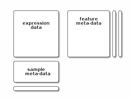
A common design theme that is found throughout many Bioconductor core classes is illustrated below, which is found in microarrays, quantiative proteomics data, RNA-Seq data, … It contains a rectangular feature x sample data matrix and sample and feature-specific annotations.
12.7 More resources
- Videos: https://www.youtube.com/user/bioconductor
- Community Contributed Help Resources: https://bioconductor.org/help/community/
- Tutorials: https://support.bioconductor.org/t/Tutorials/
12.8 Challenges
Install a Bioconductor package of your choice, discover the vignette(s) it offers, open one, and extract the R code of it.
Find a package that allows reading raw mass spectrometry data and identify the specific function. Either use the biocViews tree, look for a possible workflow, or look in the common methods and classes page on the Bioconductor page.